Running head: META-ANALYSIS

Comparison of Two Random-Effects Methods of Meta-Analysis

Michael T. Brannick

University of South Florida

Steven M. Hall

Embry-Riddle Aeronautical University

Poster presented at the 16th annual conference of the Society for Industrial and Organizational Psychology, San Diego, April 2001.

Abstract

Monte Carlo methods were used to compare the Schmidt-Hunter method of meta-analysis with the method described by Hedges and Vevea (1998). We examined the accuracy of estimates of the mean, standard deviation and credibility intervals of underlying (true, unattenuated) correlations for both methods. The Schmidt-Hunter estimates were more accurate except when the number of studies and population variance of effect size were small.

In recent years, the random-effects methods of meta-analysis have become increasingly popular (Erez, Bloom, & Wells, 1996; Hedges & Vevea, 1998; National Research Council, 1992; Overton, 1998). Random-effects methods assume that the distribution of effect sizes in the population of studies has a variance due to factors other than sampling error. Such methods provide ways to estimate the mean and variance of effect sizes excluding sampling error, that is, they allow one to estimate the mean and variance of effect sizes that one would expect if all studies had infinite sample sizes. Because such methods form the bases for theoretical positions such as validity generalization and are used in many different types of meta-analysis, differences among the methods could lead to different conclusions about a given domain. Such differences, therefore, are important to examine.

The random-effects method of meta-analysis most familiar to industrial and organizational psychologists was developed by Schmidt and Hunter (1977) and the current version is described in detail by Hunter and Schmidt (1990). In the Schmidt-Hunter method, the analyst computes the weighted mean correlation, and a weighted observed variance about this mean. Then the analyst subtracts estimated variance due to statistical artifacts such as sampling error, measurement reliability, and range restriction. The residual variance provides an initial estimate of the variance of effect sizes due to situational or context differences. The mean observed correlation and residual variance are then adjusted for attenuation due to artifacts to obtain population estimates of the mean and variance of the underlying distribution of effect sizes.

There are other methods of random-effects meta-analysis that directly estimate the variance of the effect sizes rather than estimating the variance by subtraction (Erez et al., 1996; Hedges & Vevea, 1998; Overton, 1998). It is possible that the newer methods may yield more accurate estimates of the mean and standard deviation of effect sizes because they appear to avoid some of the criticisms of the statistical aspects of the Schmidt-Hunter approach. For example, Erez et al. (1996) and James, Demaree, Mulaik, and Ladd (1992) expressed concerns for different statistical reasons that the Schmidt-Hunter method would incorrectly lump situational variance into artifactual variance. Thomas (1988) expressed concern about whether subtracting artifactual variance from observed variance yielded an appropriate estimator of situational variance. Hedges and Vevea (1998, p. 493) provided this criticism for the estimate of the mean:

On the other hand, the other random-effects methods have not been developed with reliability of measures and range restriction in mind. Therefore, to the degree that such artifacts are present, we would expect the newer procedures to provide overly conservative results unless we can devise ways to incorporate artifacts into the analysis.

Our purpose, therefore, was to compare estimates computed from the two different random-effects methods, i.e., the Schmidt-Hunter (S-H) method and the Hedges-Vevea (H-V) method. For each method, we compared parameter estimates of the mean and standard deviation of true effect sizes to known parameters through Monte Carlo techniques. We could then examine the amount of bias and the size of the standard error for each method to see whether one method was generally superior to the other, or whether one method produced better estimates in some situations but worse estimates in other situations.

The formulas that we used in the Monte Carlo study for each method were taken from Hunter and Schmidt (1990) and Hedges and Vevea (1998). The interested reader is directed to those sources for explanation of the formulas. Space limits preclude development of the formulas here.

Method

A Monte Carlo data simulation was programmed using SAS/IML (SAS Institute, 1990). The following four factors were manipulated: Size of rho, amount of variance in rho, number of studies in each meta-analysis, and attenuation. A fifth factor, sample size per study, was generated as a random variable.

The following three values of rho were presented in the study: .2, .4, and .6. These are the same values used by Erez et al. (1996) and are values that are reasonable to expect in a test validation study.

The following three values for variance in rho were also presented: 0, .15, and .30. These represent a plausible range for test validation.

The number of studies included in each meta-analysis (k) was also manipulated. The following four values of k were represented: 10, 20, 50, and 100.

True correlation values in the simulation were attenuated to simulate artifactual error. The H-V model does not address attenuation due to measurement error and range restriction, potentially leading to inaccurate results. A no-attenuation condition was also simulated so that the impact of attenuation on bias and efficiency could be assessed. Attenuation due to restriction of range and criterion reliability was simulated using the assumed distributions published in Schmidt and Hunter (1977) as a range of values.

Sample size was generated as a random variable in the simulations. A distribution of sample sizes was created based on a normal distribution with mean of 125 and a standard deviation of 25. This distribution was used to randomly generate sample size values for each of the simulated studies.

The Monte Carlo simulation "built" a series of validity studies based on the parameters for each condition. The first step was to define the true rho and the true standard deviation of rho. These values were used to create a distribution of rho from which an observed r could be sampled. Because the limit of Fischer's r to z transformation when r = +/- 1.0 is infinite, a cap of r = +/- .94 was placed on the distribution of rho. The value of .94 was chosen because this is the point in the transformation function where the transformed values begin to rise quickly.

To simulate attenuation, two arrays containing the Schmidt and Hunter (1977) hypothetical distributions of criterion reliability and range restriction were created and a value from each of these distributions was randomly selected. The sampled value of rho and the population standard deviation of rho were multiplied by the randomly selected criterion reliability value to attenuate observed r for criterion unreliability. This attenuated observed r was used to generate pairs of x and y scores expressed in terms of z. The Schmidt and Hunter hypothetical distribution for range restriction was converted into a distribution representing corresponding z cut scores. A routine in the SAS IML code examined each generated x and y score pair and discarded any score pair that had an x value less than the z cut score. This process was repeated until the appropriate number of score pairs was generated. This approach to generating range restriction is similar to the one used by Callender and Osburn (1982). This direct range restriction procedure further attenuated rho and the standard deviation of rho. These attenuation procedures were eliminated during the "no attenuation present" conditions. The random number generation procedure was repeated k times and was then analyzed using the different meta-analytic procedures.

In the attenuation condition, correction of rho and standard deviation of rho was computed for both the S-H and H-V procedures. The correction procedures described by Hunter and Schmidt (1990) were used for the S-H method. We adapted these procedures to apply them to the H-V method (a detailed description of how to do so is available upon request from the senior author).

The meta-analysis simulation process was repeated 1,000 times under each condition, resulting in 1,000 estimates of rho and of variance of rho for each condition by each meta-analysis method. Bias for each of the meta-analysis methods under the different conditions was assessed by comparing the true values of rho and the standard deviation of rho with the estimated values. Less biased estimates are closer to the true values. Efficiency of the methods was evaluated by examining the amount of variability in the estimates; specifically the standard deviation of the sampling distribution was examined. The smaller the standard deviation, the more efficient the meta-analysis method is.

Results

The data from the Monte Carlo simulations are presented in Tables 1 through 5. The estimates of rho and the standard deviation of rho (SDr ) are located in the "Est" rows and the efficiencies (standard errors) of the estimates are in the "Eff" rows.

Mean. S-H procedure produced estimates that were very slightly too small (see Table 1). The H-V procedure produced very accurate estimates when SDr was zero (see Table 2). Unlike the S-H estimates, however, the H-V estimates tended to be too large as SDr increased.

Standard Deviation. When true SDr equals zero, all mean estimates of SDr were greater than zero (Tables 1 and 2). This is due to the fact that negative estimated variances were set to equal zero during the simulation. When true SDr equals zero, the H-V model has a tendency to produce larger estimates of SDr than the S-H model. Under the SDr equals .15 and .30 conditions, the S-H model underestimates the true values of SDr and the random-effects overestimates the true values of SDr .

Efficiency. The two methods appeared equivalent, especially when SDr is either 0 or .15. When SDr is .30, the S-H method was more efficient than the H-V method, except for when rho equaled .60.

Unrealistic data. The data under rho = .60 and SDr = .30 should best be ignored because it is rather unrealistic. In such a condition, underlying correlations are quite frequently above .90 and above .94, which was our cutoff point for the r to z transformation. The resulting distribution is thus pathological and unlikely to be encountered in applied work such as test validation.

Difference in units in SD. The mean values of estimated rho used for evaluating bias of the two procedures are in the same units (that is, they are both in r). Therefore the comparison between the two models on estimates of the mean is relatively straightforward. However, the values of the standard deviation of rho are not in the same units. The S-H estimates are in r, but the H-V estimates are in z. Therefore the H-V estimates should be compared to the values in Table 3 rather than to the values in the S-H model. The values in Table 3 were computed by generating population, not sample, distributions of rho. Ten thousand values of rho were generated and transformed using Hotelling's transformation and then Fisher's r to z transformation. The standard deviations of the transformed values of rho were then computed. Notice that the standard deviation values in Table 3 are larger than the nominal values of the standard deviation of rho. The H-V estimates of the standard deviation of rho presented in Table 2 are closer to the values presented in Table 3 than to the nominal values of the standard deviation of rho.

The attenuation present data is presented in Tables 4 and 5. These tables contain the estimates of rho and SDr for the S-H corrected model and the H-V uncorrected and corrected models.

Mean. The uncorrected H-V model drastically underestimated true rho across all conditions. The corrected S-H procedure slightly underestimated rho when SDr was zero and slightly overestimated rho when SDr was .15. Under the SDr equals .30 conditions, the S-H method substantially overestimated rho. The H-V model produced very accurate estimates of rho when SDr equals zero but substantially overestimated rho in the SDr equals .15 and .30 conditions. Comparing the estimates presented in Tables 1 and 2 with those presented in Table 5, the corrected H-V estimates of rho were similar to the uncorrected estimates of rho in the no-attenuation conditions (this indicates that the correction appears to work properly).

Standard deviation. As with the no-attenuation conditions, when true SDr equals zero, all mean estimates of SDr were greater than zero. This is due to the fact that negative estimated variances were set to equal zero during the simulation. When true SDr was greater than zero, the uncorrected H-V model underestimated SDr while the corrected H-V model overestimated SDr . This tendency for the corrected H-V model to overestimate SDr became greater as true rho increased in magnitude. The corrected S-H model produced the most accurate estimates of SDr of the three models presented, but overestimation tended to occur as rho became larger.

Efficiency. The uncorrected H-V model was much more efficient than the corrected Schmidt and Hunter and corrected H-V (at the cost of considerable bias). This is due to the division of the estimated standard deviation of rho by the compound correction factor in the corrected models. The corrected models were very similar in terms of efficiency. One model did not appear to be consistently more efficient than the other.

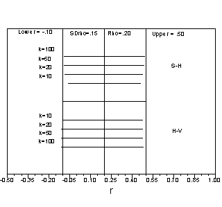
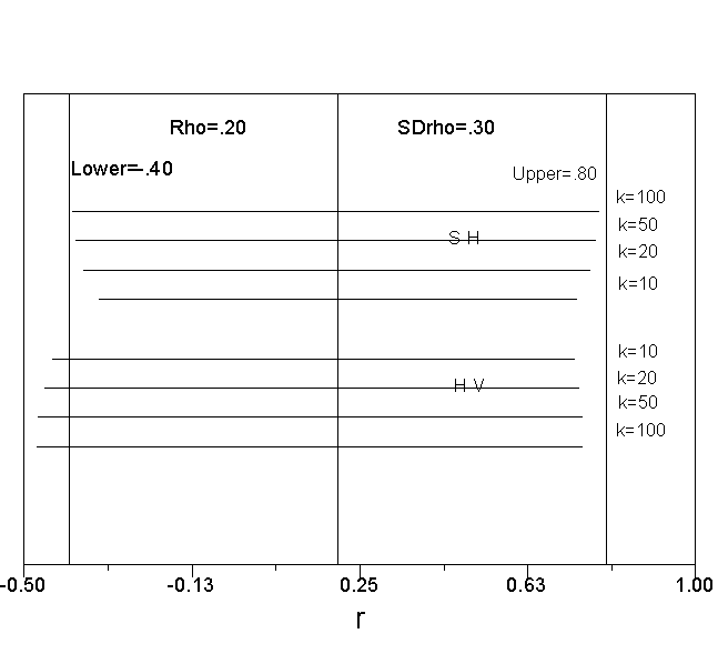
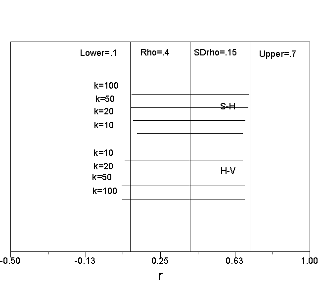
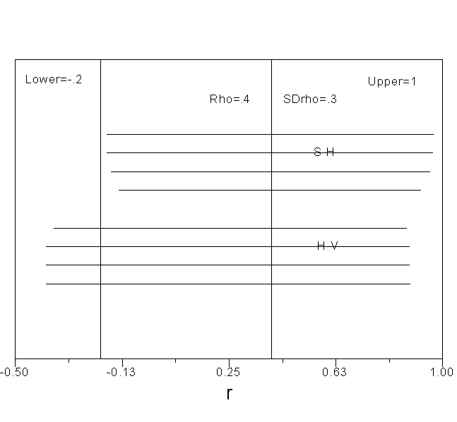
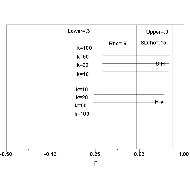
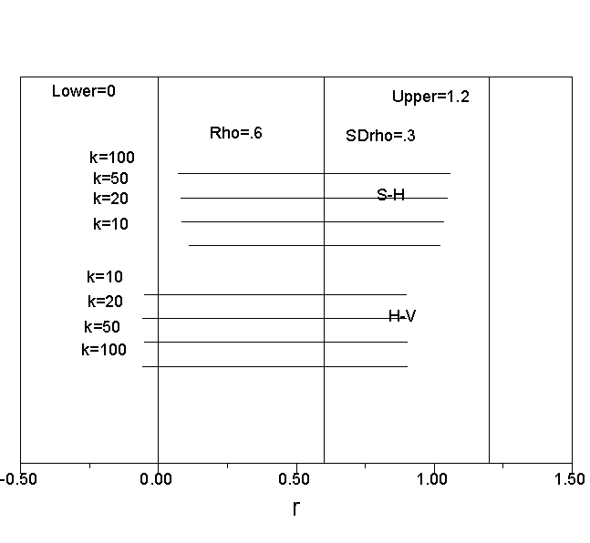
Because the H-V estimates are in z rather than r, it is difficult to compare the results of the two methods. However, it is possible to compare the results of the two models in the same units by computing credibility intervals. For the S-H model, credibility intervals were computed by taking the mean estimate of rho and then adding and subtracting 2 times the value of the estimated standard deviation (approximate 95 percent credibility interval). For the H-V credibility interval, we found the mean estimate in z, and added and subtracted 2 times the estimated standard deviation in z. This provided a credibility interval in z. We translated this interval back into r, so that the two intervals would be directly comparable. The numbers needed to do this are taken directly from Tables 1 and 2. The results are shown in Figures 1 through 6.

As can be seen in the Figures, the S-H estimates are centered on the population value of rho, and tend to approach the correct values as the number of studies (k) increases. The H-V values tend to be too low, that is, both the upper bound and lower bound of the credibility intervals tend to be too low. The only time that the H-V credibility interval appears preferable is when both the number of studies is small and the true variance of effect sizes is small.

Discussion

Monte Carlo techniques were used to compare the results of two methods of random-effects meta-analysis, the Schmidt-Hunter (S-H) and Hedges-Vevea (H-V) methods. Each method of meta-analysis was used to produce estimates of the mean rho and the standard deviation of rho in a population of studies given a sample of studies.

Regarding the mean. We found that neither method produced unbiased estimates of the mean. However, the S-H results were generally closer to the input parameter than were the H-V estimates. Estimates of the mean became increasingly inaccurate as the variance of effect sizes in the population increased.

Regarding the standard deviation. There was a problem interpreting the standard deviation estimates provided by the H-V estimates because such estimates are in z units rather than r units. Both methods appeared to produce reasonable estimates when compared to the appropriate parameters. Credibility intervals based on both the mean and standard deviation tended to favor the S-H method.

Efficiency. The standard error of the estimates provided by both models appeared approximately equal. Neither model was superior in terms of efficiency.

It proved possible to incorporate adjustments for artifacts into the H-V method to yield better estimates when unreliability and range restriction are present.

Of the two models studied here, the S-H method appears preferable overall, despite criticisms of the statistical foundation of the method. Because the results of the models were similar, inferences based on credibility values generated by either model would be the same in the vast majority of cases (see Figure 1 through 6). Of course, because of our method, our conclusions properly hold only to the type of data we simulated. The assumptions underlying both types of models were met to the limits of the number generation software. Future research might explore situations in which the models' assumptions are not met.

References

Callender, J. C. & Osburn, H. G. (1982). Multiplicative validity generalization model: Accuracy of estimates as a function of sample size and mean, variance, and shape of the distribution of true validities. Journal of Applied Psychology, 67, 859-867.

Erez, A., Bloom, M. C., & Wells, M. T. (1996). Using random rather than fixed effects models in meta-analysis: Implications for situation specificity and validity generalization. Personnel Psychology, 49, 275-306.

Hunter, J. E. & Schmidt, F. L. (1990). Methods of Meta-Analysis: Correcting Error and Bias in Research Findings. Newbury Park, CA: Sage Publications.

Hedges, L. V. & Vevea, J. L. (1998). Fixed- and random-effects models in meta-analysis. Psychological Methods, 3, 486-504.

James, L. R., Demaree, R. G., Mulaik, S. A., & Ladd, R. T. (1992). Validity generalization in the context of situational models. Journal of Applied Psychology, 77, 3-14.

National Research Council (1992). Combining information: Statistical issues and opportunities for research. Washington, DC: National Academy Press.

Overton, R. C. (1998). A comparison of fixed-effects and mixed (random-effects) models for meta-analysis tests of moderator variable effects. Psychological Methods, 3, 354-379.

SAS/IML Software: Usage and Reference, Version 6. (1990). Cary, NC: SAS Institute.

Schmidt, F. L., & Hunter, J. E. (1977). Development of a general solution to the problem of validity generalization. Journal of Applied Psychology, 62, 529-540.

Thomas, H. (1988). What is the interpretation of the validity generalization estimate S^2r = S²_r - S²_e? Journal of Applied Psychology, 73, 679-682.

Table 1

S-H estimates of rho and the standard deviation of rho for the no-attenuation condition

Table 2

H-V estimates of rho and the standard deviation of rho for the no-attenuation condition

Table 3

Expected values of rho and the standard deviation of rho for the H-V method after transformation

Table 4

Estimates of rho and efficiency for the attenuation present conditions

Table 5

Figure Captions

Figure 1. Credibility intervals when rho = .20 and SDrho = .15.

Figure 2. Credibility intervals when rho = .20 and SDrho = .30.

Figure 3. Credibility intervals when rho = .40 and SDrho = .15.

Figure 4. Credibility intervals when rho = .40 and SDrho = .30.

Figure 5. Credibility intervals when rho = .60 and SDrho = .15.

Figure 6. Credibility intervals when rho = .60 and SDrho = .30.