Running head: CORRECTING BIAS

Reducing Bias in the Schmidt-Hunter Meta-analysis

Michael T. Brannick

University of South Florida

Steven M. Hall

Embry-Riddle Aeronautical University

Poster presented at the 16th annual conference of the Society for Industrial and Organizational Psychology, San Diego, April 2001.

Abstract

The Schmidt-Hunter method of meta-analysis tends to over-estimate the amount of variance due to sampling error. We introduce a simple correction for the number of studies in the meta-analysis. Monte-Carlo simulation is used to compare unit-weighted, Schmidt-Hunter uncorrected, and Schmidt-Hunter corrected variance estimates. With small numbers of studies, the corrected formula is appreciably less biased than the original.

Reducing Bias in the Schmidt-Hunter Meta-analysis

Meta-analysis refers to the quantitative analysis of multiple study outcomes to reach conclusions regarding a body of research. Several distinct methods of meta-analysis are available (Bangert-Drowns, 1986). In recent years, increasing attention has been paid to random-effects meta-analysis methods (e.g., Erez, Bloom, & Wells, 1996; Hedges & Vevea, 1998; National Research Council, 1992; Overton, 1998). Random-effects models assume that effect sizes vary across study conditions. Random-effects models also provide mechanisms to estimate parameters of the distribution of effect sizes across study conditions.

The most popular type of random-effects meta-analysis for industrial and organizational psychologists has been the method developed by Schmidt, Hunter, and colleagues (e.g., Hunter & Schmidt, 1990; Schmidt & Hunter, 1977; Schmidt, Hunter, Pearlman & Shane, 1979; Schmidt et al., 1993). The basic idea in the Schmidt-Hunter approach is to estimate the variability of the distribution of effect sizes through a two-step process (Hunter & Schmidt, 1990). In the first step, the total variance of observed study outcomes is estimated, and the variance due to artifacts such as sampling error, reliability of measurement and range restriction is subtracted to yield a residual variance. In the second step, the residual variance is boosted by a function of the reliability and range restriction distributions to yield an estimate of the population variance of effect size.

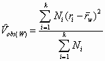
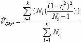
In the Schmidt-Hunter "bare bones" approach, only sampling error is considered as a source of artifactual variance. In such a case, the estimate of the variability of the study outcomes in the population is simply the difference between the estimated variance of observed studies and the estimated variance of sampling error; the second step mentioned above is omitted. The formula offered by Hunter and Schmidt (1990) for the observed variance is:

, (1)

where there are k studies, N_i is the sample size for the ith study, r_i is the observed correlation for the ith study, and is the weighted mean correlation across studies. The carat (hat) above the V indicates an estimate of a population parameter, namely the weighted estimate of observed variance. The weighted mean is computed by:

. (2)

Hunter and Schmidt (1990) used the following formula to estimate the variance due to sampling error:

, (3)

where is the mean sample size across studies. The Hunter and Schmidt (1990) estimate of the variance in effect sizes in the bare bones case is simply the difference between Equations 1 and 3, thus:

. (4)

The expectation is that when the variance of effect sizes in the population is zero, then the variance observed will equal the variance due to sampling error. Therefore, when one subtracts the variance due to sampling error from the variance observed, one should get a result of zero (in practice, about half of the time the result should be positive and half of the time the result should be negative due to having a finite number of studies).

A problem occurs in Equation 3 when Vr > 0 (Erez et al., 1996). The larger the Vr , the more Equation 3 overestimates sampling error, and the more is underestimated. However, the amount of bias introduced by using Equation 3 is small. One can instead use the following for an estimate that is less biased:

(5)

The price to be paid for the reduction in bias in a reduction in efficiency. The individual values of r are poorer estimates of the r _i than is the mean r for average r . In this paper, we consider a different source of bias in greater detail.

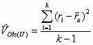
Consider instead unit weighted estimates of the mean and variance of the observed study effect sizes (Osburn & Callender, 1992; Thomas, 1988). The mean would be calculated as

, (6)

where is the unit weighted mean correlation, and k is the number of studies. The unit weighted variance would be:

, (7)

where the terms on the right side of Equation 6 have been defined previously. One might think that the variances produced by Equations 1 and 6 would be the same when the samples sizes N_i are all equal. Such is not the case, however, because Equation 1 is a descriptive variance rather than an inferential variance. In other words, Equation 6 adjusts the variance for the number of studies, but Equation 1 does not. The result is that for small numbers of studies, Equation 1 results in an appreciably biased estimate of the observed variance. The bias produces a mean estimate of the variance of effects sizes (Vr ) that is too small, resulting in credibility intervals that are too small.

A simple correction for such a problem is to compute a corrected observed variance estimate by:

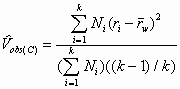, (8)

where the terms on the right of Equation 7 have been defined previously. Equation 7 yields results equal to those of Equation 6 when the N_i are all equal. When the N_i are unequal, Equation 7 produces results that are less biased than Equation 1, as we show in the next section, which is a Monte Carlo study.

Method

SAS IML was used to generate distributions of correlation coefficients under several conditions. The factors that we varied were the variance in sample size per study (V_N), and the number of studies per meta-analysis (k). For each study, the population correlation (r ) was set at .40. The mean sample size was set at 120. The standard deviation in sample size systematically varied using the values 0 (all samples of size 120), 25, 50, or 75. A random number generator was instructed to sample a value of N from a normal distribution with a mean of 120 and a standard deviation of 0, 25, 50 or 75. The program was instructed to set a minimum sample size at 15. If the sample size was less than 15, the program sampled another number at random until the result was greater than or equal to 15.

The number of studies per meta-analysis was set at 5, 10, 25, and 100. For each combination of studies and variance of N, one thousand meta-analyses were simulated. For each condition across all meta-analyses, Equation 3 was used to compute the expected sampling error of the distribution of correlation coefficients. That is, the values of and were computed across all studies in a given condition rather than within each meta-analysis. This was done to insure that the estimated sampling error variance would be very accurate.

For each meta-analysis within each condition, three estimates of the observed standard deviation were calculated. The first was a unit-weighted standard deviation computed as the square root of Equation 6. Next was the Schmidt-Hunter standard deviation, computed as the square root of Equation 1. Finally, the k-corrected Schmidt-Hunter standard deviation was computed as the square root of Equation 7.

Analyses and Results

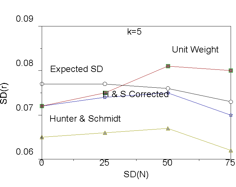
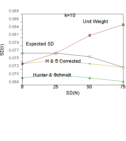
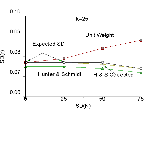
For each condition (variance of N and number of studies, k) we computed the mean of the sampling distribution for each of the three methods of estimating the observed standard deviation (unit weight, Schmidt-Hunter uncorrected, and Schmidt-Hunter k-corrected). We also computed the expected variance due to sampling error overall for each condition. Results for k = 5, 10, and 25 are shown graphically in Figures 1 through 3.

First consider the values for the expected standard deviation due to sampling error computed by Equation 3. The values are shown in each Figure as open circles. The expected value of sampling error serves as a benchmark. To yield an unbiased estimate of Vr , the estimate of the observed standard deviation should equal the expected standard deviation by sampling error. The reason that the expected standard deviation by sampling error decreases as the standard deviation of N increases is that the distribution of N becomes increasingly skewed as the standard deviation of N increases, so that average N increases and therefore expected sampling error decreases (see Equation 3). So, for example, when the standard deviation of N is zero, then the average N is 120, but when the standard deviation of N is 75, then the average N is about 135.

As can be seen in Figure 1, when there are five studies in the meta-analysis, unit weights provide under-estimates of observed variance when N is similar across studies, but over-estimates of observed variance when N is dissimilar across studies. As previously mentioned, the unit weighted and corrected Schmidt-Hunter estimates are equal when N does not vary across studies. Figure 1 also shows that both the Schmidt-Hunter corrected and uncorrected estimates are too small on average, thus yielding biased estimates of Vr . Note that the magnitude of bias is appreciable (about .10) for the Schmidt-Hunter uncorrected estimate, but less so (about .002) for the Schmidt-Hunter corrected estimate. Put another way, the Schmidt-Hunter estimate is about 87 percent as large as it should be, and the k-corrected Schmidt-Hunter estimate is about 97 percent as large as it should be. When there are 10 studies per meta-analysis, the Schmidt-Hunter uncorrected and corrected estimates are 92 and 98 percent as large as they should be. When there are 25 studies, the Schmidt-Hunter corrected estimates are essentially unbiased.

As we move from five studies (Figure 1) to 10 and 25 studies (Figures 2 and 3), we can see that the Schmidt-Hunter estimates approach the standard deviation expected due to sampling error. The Schmidt-Hunter uncorrected estimates become closer to the corrected estimates. As the number of studies increases, the unit weighted standard deviation becomes too large. At 100 studies per meta-analysis, the Schmidt-Hunter corrected, uncorrected and expected standard deviation are all virtually identical. At 100 studies per meta-analysis, unit weights only provide unbiased estimates when N does not vary across studies.

Because we chose a single value for rho (.40) and N (120), there remains some question about whether the same pattern of results would obtain for other values of rho and N. The absolute magnitude of the bias will depend upon both and . As and increase, the absolute magnitude of the bias will decrease. However, the proportion of bias will remain approximately constant. In other words, meta-analyses based on five studies using the Schmidt-Hunter uncorrected observed variance estimate will produce estimates about 80 percent as large as they should be on average. Studies based on ten studies will produce variance estimates about 90 percent as large as they should be on average.

Discussion

For small numbers of studies in a meta-analysis, the Schmidt-Hunter estimate of observed variance is too small, leading to biased estimates of Vr . Using a simple correction substantially reduces the amount of bias, leading to better meta-analytic estimates. Users of the Schmidt-Hunter procedure should employ the correction, particularly if the number of studies in the meta-analysis is small. Overton (1998) made a similar point with regard to the iterative random-effects variance estimates described by Erez et al. (1996).

One may question our use of a single population value of r considering that a random-effects meta-analysis assumes that r has a distribution with some mean and variance (that is, in our simulation, Vr was set to zero). Although it is true that the practical result of the bias is to cause the Schmidt-Hunter estimate of Vr to be too small on average, the point of the current paper is to show that the average value of Equation 1 is too small even when the assumption that r has only one value is correct, so that Equation 3 should properly apply. Thomas (1988) also criticized the Schmidt-Hunter estimates based on the expected values of formulas slightly different than those presented here. However, Thomas used an observed variance formula that adjusts for the number of studies, and the magnitude of the difference between observed variance and variance expected by sampling error was much smaller than that reported here (e.g., in his study with r equal to .4 and N_i at 50, the expected difference was .000442).

The point of this paper would be primarily of academic interest if meta-analyses were exclusively computed on large numbers of studies. However, such is not the case, as even a cursory inspection of the literature reveals. In some cases there are few studies of interest that can be sampled. For example, Brown (1981) was interested in a test validation in the life insurance industry. He found 12 studies. For another example, Wright, Lichtenfels, and Pursell (1989) meta-analyzed a total of 13 studies of the validity of structured interviews for predicting job performance. Levine, Spector, Menon, Narayanan, and Cannon-Bowers (1996) computed meta-analysis on as few as six validation studies. Sackett, Harris, and Orr (1986, p. 303) pointed out that meta analysis in research areas in induustrial and organizational psychology other than test validation are often carried out with numbers of studies less than 25. Drug trials in medicine is another area in which there may be few studies to combine (e.g., LeLorier, Gregoire, Benhaddad, Lapierre, & Derderian, 1997).

More often, researchers start with a large number of studies and then split them into smaller groupings to search for moderators or to examine the effects of excluding certain types of studies. For example, Tett, Jackson, and Rothstein (1991) collected 97 studies in which personality measures were used to predict job performance. In addition to a meta-analysis based on all 97 correlations, they computed 18 different meta-analyses of specific interest. Of these 18, six were based on fewer than 25 studies and two were based on fewer than ten studies. They then broke one of the categories into nine subcategories for subsequent analysis. All nine were based on fewer than 25 studies; one of these was based on two studies. It appears that small numbers of studies for a meta-analysis are quite common. Therefore, the correction has applied as well as theoretical benefits.

References

Bangert-Drowns, R. L. (1986). Review of developments in meta-analytic method. Psychological Bulletin, 99, 388-399.

Erez, A., Bloom, M. C., & Wells, M. T. (1996). Using random rather than fixed effects models in a meta-analysis: Implications for situational specificity and validity generalization. Personnel Psychology, 49, 275-306.

Hedges, L. V., & Vevea, J. L. (1998). Fixed- and random-effects models in meta-analysis. Psychological Methods, 3, 486-504.

Hunter, J. E., & Schmidt, F. L. (1990). Methods of meta-analysis: Correcting error and bias in research findings. Newbury Park, CA: Sage.

LeLorier, J., Gregoire, G., Benhaddad, A, Lapierre, J., & Derderian, F. (1997). Discrepancies between meta-analyses and subsequent large randomized, controlled trials. New England Journal of Medicine, 337, 536-542.

Levine, E. L., Spector, P. E., Menon, S., Narayanan, L., & Cannon-Bowers, J. (1996). Validity generalization for cognitive, psychomotor, and perceptual tests for craft jobs in the utility industry. Human Performance, 9, 1-22.

National Research Council (1992). Combining information: Statistical issues and opportunities for research. Washington, DC: National Academy Press.

Overton, R. C. (1998). A comparison of fixed-effects and mixed (random-effects) models for meta-analysis tests of moderator variable effects. Psychological Methods, 3, 354-379.

Sackett, P. R., Harris, M. M., & Orr, J. M. (1986). On seeking moderator variables in the meta-analysis of correlational data: A monte carlo investigation of statistical power and resistance to Type I error. Journal of Applied Psychology, 71, 302-310.

Schmidt, F. L., & Hunter, J. E. (1977). Development of a general solution to the problem of validity generalization. Journal of Applied Psychology, 62, 529-540.

Schmidt, F. L., Hunter, J. E., Pearlman, K., & Shane, G. S. (1979). Further tests of the Schmidt-Hunter Bayesian validity generalization procedure. Personnel Psychology, 32, 257-281.

Schmidt, F. L., Law, K., Hunter, J.E., Rothstein, H. R., Pearlman, K., & McDaniel, M. (1993). Refinements in validity generalization methods: Implications for the situational specificity hypothesis. Journal of Applied Psychology, 78, 3-12.

Tett, R. P., Jackson, D. N., & Rothstein, M. (1991). Personality measures as predictors of job performance: A meta-analytic review. Personnel Psychology, 44, 703-741.

Thomas, H. (1988). What is the interpretation of the validity generalization estimate ? Journal of Applied Psychology, 73, 679-682.

Wright, P. M., Lichtenfels, P. A., & Pursell, E. D. (1989). The structured interview: Additional studies and a meta-analysis. Journal of Occupational Psychology, 62, 191-199.

Figure Captions.

Figure 1. Results for k=5 studies.

Figure 2. Results for k=10 studies.

Figure 3. Results for k=25 studies.