Continuous and Categorical IVs 1
Objectives
When we model a single categorical and a single continuous variable, what do the main effects look like? What do the interactions look like?
What is the meaning of each of the three b weights in such models?
What is the sequence of tests used to analyze such data?
Why should we avoid dichotomizing continuous IVs?
What is the difference between ordinal and disordinal interactions?
Why do we test for regions of significance of the difference between regression lines when we have an interaction?
What is the Equal Risk Model definition of a biased test?
What is the Cleary Model definition of a biased test?
How does reliability affect the detection of test bias?
Materials
Modeling both Categorical and Continuous Variables
We have analyzed data with one or more categorical variables (race, sex, marital status) and with one or more continuous variables (test scores, time since trial, drug dosage). Now we consider analyzing data that contains both continuous and categorical independent variables at once. We will assume a continuous dependent variable, as we have throughout. Models in which there are both continuous and categorical variables are often called analysis of covariance or ANCOVA for short.
To begin, let's consider the simplest model of this sort possible. Then we will build generalizations of it. Suppose we have:
Suppose our data look something like this:
|
N |
Sex |
MAT |
GPA |
N |
Sex |
MAT |
GPA |
|
1 |
1 |
51 |
3.7 |
21 |
-1 |
47 |
2.72 |
|
2 |
1 |
53 |
3.28 |
22 |
-1 |
53 |
3.62 |
|
3 |
1 |
52 |
3.79 |
23 |
-1 |
51 |
3.45 |
|
4 |
1 |
50 |
3.23 |
24 |
-1 |
51 |
3.78 |
|
5 |
1 |
54 |
3.58 |
25 |
-1 |
46 |
3.14 |
|
6 |
1 |
50 |
3.34 |
26 |
-1 |
48 |
2.89 |
|
7 |
1 |
52 |
3.05 |
27 |
-1 |
51 |
3.36 |
|
8 |
1 |
56 |
3.78 |
28 |
-1 |
51 |
3.05 |
|
9 |
1 |
49 |
3.23 |
29 |
-1 |
53 |
3.65 |
|
10 |
1 |
52 |
3.16 |
30 |
-1 |
55 |
3.61 |
|
11 |
1 |
50 |
3.46 |
31 |
-1 |
50 |
3.45 |
|
12 |
1 |
51 |
3.47 |
32 |
-1 |
51 |
3.43 |
|
13 |
1 |
49 |
3.73 |
33 |
-1 |
52 |
3.56 |
|
14 |
1 |
54 |
3.63 |
34 |
-1 |
50 |
3.14 |
|
15 |
1 |
48 |
3.09 |
35 |
-1 |
49 |
3.19 |
|
16 |
1 |
48 |
3.18 |
36 |
-1 |
49 |
3.32 |
|
17 |
1 |
53 |
3.58 |
37 |
-1 |
50 |
3.06 |
|
18 |
1 |
53 |
3.26 |
38 |
-1 |
52 |
3.47 |
|
19 |
1 |
48 |
3.11 |
39 |
-1 |
44 |
3.07 |
|
20 |
1 |
47 |
3.22 |
40 |
-1 |
52 |
3.66 |
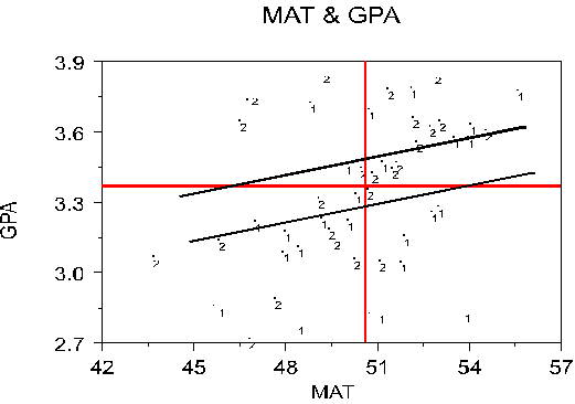
Note that there are 40 people here; the first four columns are one set of data and the second four columns are another; the data are concatenated horizontally so that all 40 will fit on single page. Effect coding for sex.
Telling the story with graphs
A graph of the data might look like this:
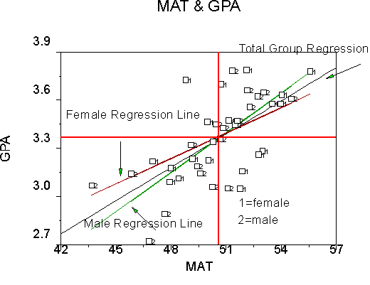
As is typical of data analysis, the graph tells most of the story that the data have to offer. We can estimate a regression line for the total group including everybody and ignoring the group distinction. This is shown with the total group regression line; the slope is called the common regression coefficient or common slope. We can also estimate a regression line for each group excluding the members of the other group. This is shown here as a male regression line and a female regression line. (The data are effect coded so that male = "-1" in the table but "2" in the graph.)
A digression on the common regression coefficient. The common regression coefficient has this relation to the coefficients in the groups:
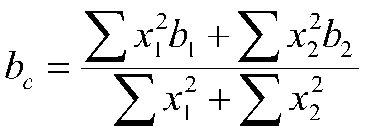
This equation says that the common slope is the weighted average of the group slopes (this formula generalizes to any number of groups). If the sum of squares is the same for the groups, then the common slope is the simple average of the b weights. (e.g., (1b1+1b2/(1+1) = (b1+ b2)/2=average). If the sums of squares X (S x2) across groups are different, then the group bs are weighted for each group by that group's sum of squares. We add the weighted b weights and divide by the total sum of squares, resulting in a weighted average. Note that two things affect the size of the sum of squares: the variability of X in that group, and the number of people in that group. Influential groups tend to have lots of variability on X and lots of people in their group. Back to the graph.
Here, for example, it appears that both groups show pretty much the same relations between MAT and GPA (although the lines are not identical in the sample, they may be in the population). Of course, statistical tests are needed to confirm what the eye seems to detect. With data such as these, we conduct a sequence of tests to determine the facts behind the story. But before I show you the sequence of tests, let's look at what the possible stories are, from the simplest to the most complex.
First, we could have no story to tell, where there is no difference between groups and no relations between the continuous IV and the DV.
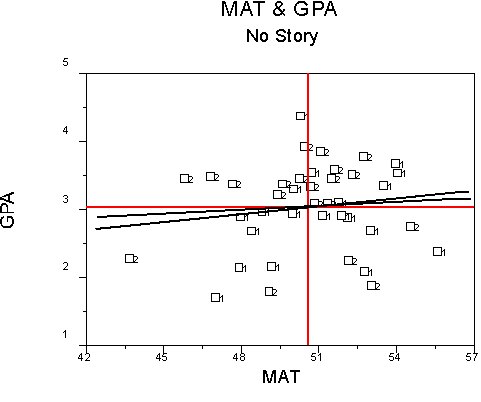
Note that both lines are essentially horizontal (zero slope) and that the intercept values are about the same for both lines. This means that MAT is unimportant for either group and that the groups do not differ from one another in GPA.
There are two possible single stories: One for the continuous variable, and one for the categorical variable. The story for the continuous variable:
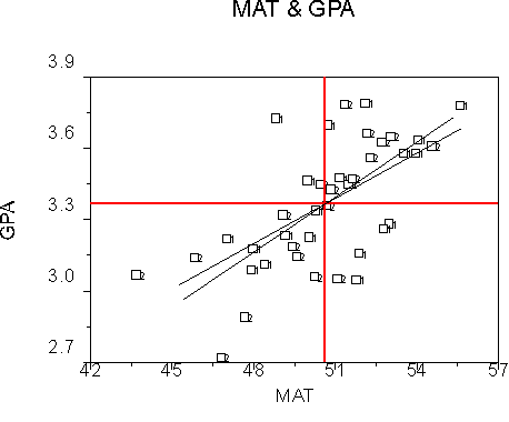
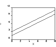
Note that the slopes for both groups are positive and that the intercepts will be nearly identical (well, pretend it's so). The continuous IV is the story because it seems to have an effect, but the group variable does not.
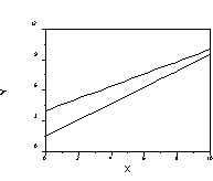
The other single story is an effect of the group variable only. It might look like this:
Note that the slopes for both groups are about zero, but the groups differ in GPA.
Of course, both IVs could be influential. In that case, we would expect both substantial slopes, and different intercepts, such as this one:
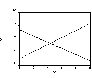
Finally, there could be truly different relations between X and Y for each group. This would be in interaction between X and Group membership in producing Y. For example:
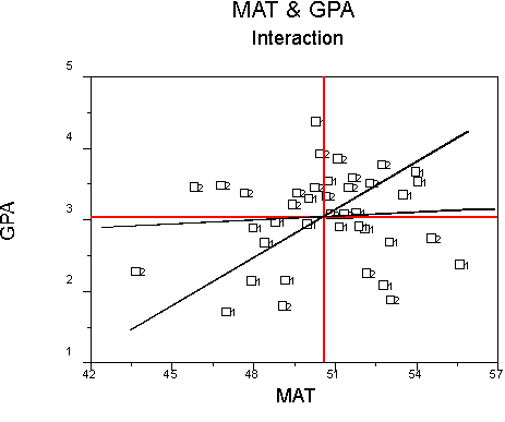
Note that for one group, there is essentially no relation between MAT and GPA, but for the other group, there is a substantial relation between MAT and GPA. This is an interaction because the relations between X and Y (regression of Y on X or effect of X on Y) depend upon the value of G. Note also that other interactions could be found in addition to the one shown here. For example, the slope could be positive for one group and negative for the other group. To model this kind of interaction, we can compute separate regressions, one for each group.
Now you should have an idea through graphs how to tell the story the data have to offer. But what graph is truly best? How to decide?
Testing Sequence
First, construct a vector to represent the continuous variable, MAT. Let's call that vector X, for a continuous variable. Let's construct a vector for the group membership, and call it G for group (suppose for the moment that we construct it as an effect code with1 for female and -1 for male. Finally we construct a vector for the interaction between
G and X We simply multiply G and X to get the vector GX (subtract the mean of X first if you wish). Now we can write the regression equation:
![]()
Note that we only need to estimate the intercept and three b weights. The intercept and the b weights correspond to particular parts of the graph. Two parts of this equation refer to the total group without reference to the subgroups. The intercept, a, refers to the total group intercept. The regression weight b2 refers to the total group regression of Y on X (in our case, GPA on MAT). The weight b2 tells whether the common slope (the slope for the whole group modeled at once, ignoring group membership) is positive, negative, or zero.
The other two parts refer to differences in the first two (intercept & slope) due to group membership. The first b weight (b1) adjusts the intercept for each group. That is, b1 determines whether each group's intercept should be moved up or down compared to the total group (at least for effect coding). The third b weight (b3) is for the homogeneity of slopes, that is, it adjusts the common slope up or down, depending on the group membership. Any adjustments are made on an as needed basis depending on the difference between the groups (they are least squares estimates). Together, the three b weights tell us nearly all of what we need to know to tell our story. I recommend the following three steps:
Step 1:
Compute R2 for the whole model, that is R2y.123. If it is not significant or if it is significant but too small to be meaningful, stop. The IVs don't have a story to tell.
Step 2:
Look at the significance of b3. If it is significant, compute separate regressions for each group (that is, split the data and compute slopes and intercepts for each). If it is not significant, drop the interaction term and recompute b1 and b2, then go on to the last step.
Step 3:
Look at the significance of b1 and b2.
|
|
Is b1 significant? |
|
|
Is b2 significant? |
Yes |
No |
|
Yes |
Parallel slopes, different intercepts |
Identical regressions |
|
No |
Mean differences only; slopes are zero |
Only possible with severe confounding; ambiguous story. |
Let's try an example or two to see how this works. (In practice, the sequence of tests will be slightly more complex; however, the logic is identical to the current case).
For the current data:
The results of the regression with all three variables.
|
R2 = .44; p < .05 |
|||
|
Y' = -.0389+.75G+.0673X-.0146GX |
|||
|
Term |
Estimate |
SE |
t |
|
G (b1; Sex) |
.75 |
.6856 |
1.0567 |
|
X (b2; MAT) |
.0673 |
.0125 |
4.9786* |
|
GX (b3; Interaction) |
-.0146 |
.0135 |
-1.0831 |
Step 1: Note that R2 is large and significant.
Step 2: Note that b3 (for GX) is not significant. This means that there is no interaction; the slopes for the two groups are not significantly different. Therefore, let's drop the interaction term and go back and re-estimate the other two.
[Technical note: The p value for the interaction was p = .286 (not shown earlier). Pedhazur recommends a liberal alpha, such as .10 or .20 for this term be used because we are essentially accepting the null hypothesis as true when we re-estimate the other two weights. The test for the difference between slopes is not very powerful in most circumstances.]
Step 3:
|
R2 = .42; p < .05 |
|||
|
Y' = .1154+.0045G+.0687X |
|||
|
Term |
Estimate |
SE |
t |
|
G (b1; Sex) |
.0045 |
.0833 |
.1365 |
|
X (b2; MAT) |
.0687 |
.0135 |
5.0937* |
Here we find that the term for the slope of MAT is significant, but the term for the group is not. This result means identical regressions.
That is, both groups show the same regression (same slope, determined in step 2; same intercept, determined in step 3). This result agrees with our original graph interpretation.
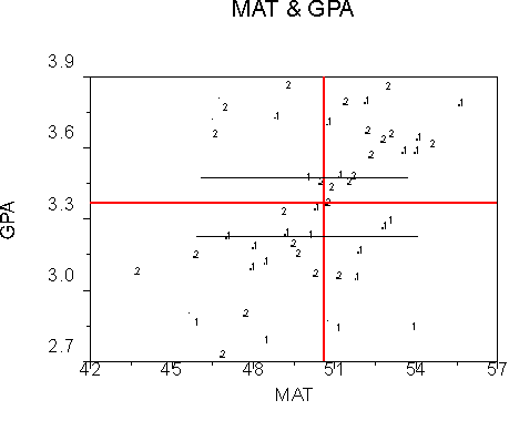
Suppose instead that our data look like this:
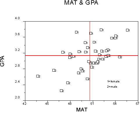
Look at the positions of the 1s and 2s. What story does this graph tell you?
Let's analyze the data using effect coding for the categorical variable.
For the first analysis, we have
|
R2 = .72; p < .05 |
||||
|
Y' = -11.54+.8268G+.0643X-.0117GX |
||||
|
Term |
Estimate |
SE |
t |
p |
|
G (b1; Sex) |
.8268 |
.6627 |
1.2476 |
.22 |
|
X (b2; MAT) |
.0643 |
.0131 |
4.2947 |
.0001 |
|
GX (b3; Interaction) |
-.0117 |
.0131 |
-.8945 |
.3770 |
Note that the R2 is significant and large.
The term for the interaction is not significant, indicating common slopes. Therefore, we re-estimate the first two terms:
|
R2 = .72; p < .05 |
||||
|
Y' = -.1805+.2346G+.0655X |
||||
|
Term |
Estimate |
SE |
t |
p |
|
G (b1; Sex) |
.2346 |
.0320 |
7.34 |
.0001 |
|
X (b2; MAT) |
.0655 |
.0130 |
5.05 |
.0001 |
Here we see that both common slope and differential intercept terms are significant. This means that we have the parallel slopes model, that is, one slope and two intercepts for parallel regression lines, one for each group. Why do you suppose that the term for group (b1, sex) was not significant in step 2 but was significant in step 3?
More Complicated Designs
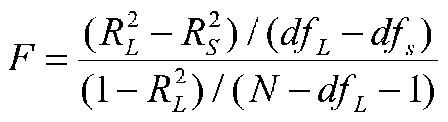
We may have a categorical variable with more than two levels. We may have more than one continuous independent variables, and so forth. In such cases, the analysis is complicated somewhat, but the logic remains the same. In designs with more than two groups, more than one product term must be generated (we need G-1 vectors). To test the interaction of the categorical variable with the continuous variable, we test the difference between the R-squares of the model with no interaction terms and the model with all (G-1) interaction terms, using the familiar hierarchical F, namely:
Categorizing Independent Variables
Some researchers split their continuous data into groups. For example, participants may respond to a stress inventory and may be placed on the basis of a median split into a high stress group and a low stress group. Or people may do median splits on more than one continuous IV. For example in the Bem Sex Role Inventory, participants respond to two scales, masculinity and femininity. On basis of median split, each person is high or low on each scale. Participants are then classified into one of four types based on the splits. If you are high masculine and low feminine, you are masculine. If you are high masculine and high feminine, you are androgynous. If you are low masculine and high feminine, you are feminine. Finally, if you are low on both, you are undifferentiated. People usually turn continuous variables into categorical ones so that they can use ANOVA instead of regression for the analysis. In most cases, they were taught ANOVA and have not learned regression. There are several reasons that you should avoid categorizing (usually dichotomizing) your continuous IV:
Even if both reasons 2 and 3 can be dealt with, reason 1 (power) remains a problem. Because you have been taught how to handle continuous data through regression, you have no need to categorize continuous variables.
There is one other situation in which people categorize their continuous variable(s). That is to throw away the middle of the distribution and to analyze only data from the highest and lowest people in the distribution (e.g., keep the upper and lower quartiles, toss the middle 50 percent). Such a practice is highly controversial. It results in a biased correlation (as I said at the beginning of the course when we were studying correlations) because of range enhancement, the opposite of range restriction. The practice might be defended when you are trying to see if something could have an effect, and not what the effect is. If you do this, you also need to be clear with your audience that your result is an overestimate of the effect of the variable. In virtually all cases, if you collect data on a continuous IV, you should analyze that as a continuous IV through regression.
Interactions
In most of psychology, main effects are the main interest (What is the most effective therapy? What is the best way to select employees?) There are some areas in psychology were interactions are of major importance, however. Instruction is one such area. Many people believe that some methods of instruction are superior for some people, while other methods are better for other people, given the same topic. Some people learn best by hearing words, for example, while others learn best by seeing pictures. People who work in this area often refer to it as the study of the Aptitude Treatment Interaction (ATI). In ATI research, it is usually the case that the categorical variable is an instructional treatment that is manipulated (e.g., lecture vs. workbook) and the continuous variable is an individual difference variable (aptitude) that is not manipulated (e.g., verbal ability, occupational interest, learning preference style). A major interest is in the interaction, so that it may be possible to pick for a person that type of instruction best suited for him or her for maximum learning, efficiency, satisfaction, etc.
Ordinal vs. Disordinal Interactions
If there is an interaction, it is either ordinal or disordinal. An ordinal interaction has the property that throughout the range under consideration, one treatment is always superior to the other (ordinally superior). In such an interaction, the regression lines do not cross. In the disordinal interaction, the regression lines cross, and in some cases, one treatment is better than a second, but in some other cases the first is worse than the second.
|
No interaction |
Ordinal Interaction |
Disordinal Interaction |
|
|
|
|
Clearly, the ordinal interaction would become disordinal if given enough range. The interaction, therefore, is only considered under the research range of interest. In educational treatments, for example, we might disregard IQ above 165 because we rarely meet such people, and if we do, they will do all right no matter what treatment they get (unless they die of boredom).
If we have a disordinal interaction, we can talk about regions of the difference where one treatment is significantly better than the other, and where there is no significant difference between the two. Clearly, at the point where the lines cross, the treatments are not different. Of course, we only know where the lines cross for our sample, and not in the population. That's why we need to talk about regions of significance. However, where the lines cross in the sample is a good bet for no difference in the population, and that's where we will start.
The way to find the point of intersection for single-variable lines is to use the slopes and intercepts
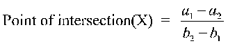
Suppose we have the following two lines:
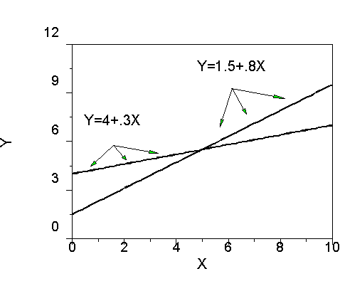
The crossover is found by (a1-a2)/(b2-b1) or (4-1.5)/(.8-.3) = 2.5/.5 =5, just where it appears to be on the graph.
Where are the treatments different and the same? To determine this, we can compute simultaneous regions of significance using formulas reported by Pedhazur:
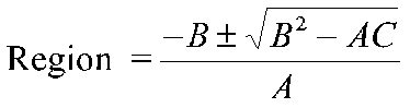
Where
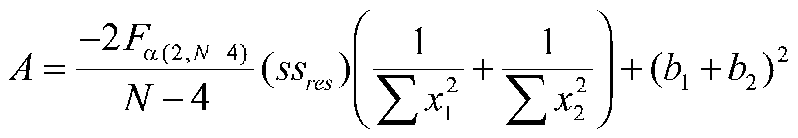
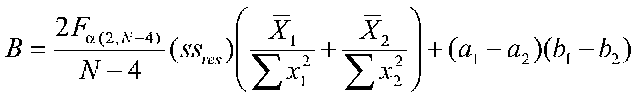
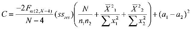
Where Fa (2,N-4) is the tabled F value with 2 and N-4 degrees of freedom at your chosen alpha level, ssres is the pooled sum of squares residual from the separate groups' regressions, N is the total sample size, n1 and n2 are the group sample sizes, the means refer to the means of each group on the continuous variable X, the sums of squares are sums of squares for each group on X, and a and b are regression intercepts and slopes.
Example of Disordinal Interaction
Suppose we have the following data:
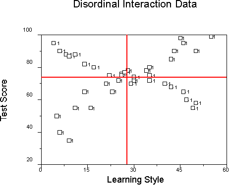
We gave students in Research Methods class a learning style questionnaire that asks them about their preference for spoken language in instruction. High scores mean that the student prefers spoken language to visual symbols. Two instructional techniques were used. One method was traditional lecture (coded 1); the other method was a tutorial presented by computer and employing written (not aural) scripts and extensive graphics (coded -1). At the end of a module of instruction, all students took the same examination, which was the garden-variety multiple choice research methods exam.
We code the continuous independent variable as X, the treatment as G, and the DV as Y. Regression shows us that for the total group (N=40):
|
R |
Y (Test) |
X (Learn Style) |
G (Lect v. tutor) |
GX (Int) |
|
Y |
1 |
|
|
|
|
X |
.22 |
1 |
|
|
|
G |
-.09 |
.03 |
1 |
|
|
GX |
.35 |
.02 |
.88 |
1 |
|
M |
73.8 |
27.78 |
0 |
.43 |
|
SD |
15.06 |
15.14 |
1.01 |
31.94 |
|
Source |
Df |
SS |
|
|
|
Model |
3 |
8035.69 |
|
|
|
Error |
36 |
806.70 |
|
|
|
C Total |
39 |
8842.40 |
|
|
|
R2=.91 |
|
|
|
|
|
Variable |
Estimate |
SE |
t |
p |
|
Intercept |
67.09 |
|
|
|
|
G |
-26.99 |
1.58 |
-17.09 |
.0001 |
|
X |
.227 |
.05 |
4.54 |
.0001 |
|
GX |
.917 |
.05 |
18.33 |
.0001 |
Note that the interaction term is significant. Therefore, we will compute separate regressions for each group. For the "1" group, we find that:
|
n1=20 |
Y |
X |
|
|
G=1 |
|
Y |
1 |
R |
|
|
|
|
X |
.95 |
1 |
|
|
|
|
M |
72.4 |
28.2 |
|
|
|
|
SD |
18.43 |
15.26 |
|
|
|
|
Source |
Df |
SS |
|
G=1 |
|
Model |
1 |
5805.09 |
|
|
|
Error |
18 |
651.71 |
|
|
|
C Total |
19 |
6456.80 |
|
|
|
R2 = .90 |
|
|
|
|
|
Variable |
Estimate |
SE |
t |
p |
|
Intercept |
40.10 |
2.88 |
13.9 |
.0001 |
|
X |
1.15 |
.09 |
12.66 |
.0001 |
For the "-1" group, we find that:
|
n2=20 |
Y |
X |
|
|
G=-1 |
|
Y |
1 |
R |
|
|
|
|
X |
-.97 |
1 |
|
|
|
|
M |
75.2 |
27.35 |
|
|
|
|
SD |
11.02 |
15.41 |
|
|
|
|
Source |
df |
SS |
|
G=-1 |
|
Model |
1 |
2152.21 |
|
|
|
Error |
18 |
154.99 |
|
|
|
C Total |
19 |
2307.20 |
|
|
|
R2 = .93 |
|
|
|
|
|
Variable |
Estimate |
SE |
t |
P |
|
Intercept |
94.09 |
1.36 |
69.03 |
.0001 |
|
X |
-.69 |
.04 |
-15.81 |
.0001 |
Therefore, the regression with all terms included is:
Y' = 67.09 - 26.99G + .23X + .92GX
The regression for the 1 group is:
Y' = 40.1 + 1.15X
The regression for the -1 group is:
Y' = 94.09 - .69X.
To find the crossover point, we find (a1-a2)/(b2-b1) which, in our case is (94.0881-40.1011)/(1.14535+.69061) = 29.41. The value of X at which the regression lines cross is 29.41. Therefore at first guess, we would say to give people with learning style scores of 30 or more the lecture and to give people with scores of 29 or less the tutorial. Note that what we are doing here is analogous to post hoc testing in ANOVA.
To do a better job of finding the simultaneous confidence intervals, we use the nasty equations described above.
|
N=40 |
n1=20 |
n2=20 |
Group1 = 1 Group2 = -1 |
|
F.05(2,36)=3.26 |
SSres(tot) = 806.70 |
SSres(1) = 651.71 |
SSres(2) = 154.99 |
|
|
Note: SSres(tot) |
= SSres(1) + |
+ SSres(2) |
|
|
SD=15.26123, SS =SD2*(n1-1) |
|
SD=15.41112, SS=SD2*(n2-1) |
|
|
From corrs |
|
From corrs |
|
a1=40.1011 |
b1=1.14535 |
a2=94.0881 |
b2=-.69061 |
![]()
![]()

![]()
![]()
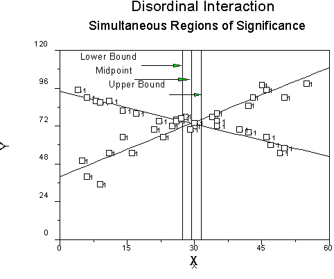
Therefore, our estimates are:
|
Lower |
27.32 |
|
Middle |
29.41 |
|
Upper |
31.55 |
The results as a graph:
Click to learn more about instructional outcomes as a function of learning styles. For the interaction, click "crossover" when you get there.
Test Bias
Tests are used to make decisions about people. If test scores don't mean what we think, there are all kinds of problems.
The difference between fairness and bias in testing.
Fairness is a value judgment about the use of a test. Reasonable people can disagree about the fairness of a test because of value differences. Bias is an evaluation of the relations between test scores and criterion scores. We have a biased test used fairly and even if a test is unbiased, some people will think it unfair if used in an unbiased manner.
The problem with mean differences
Mean differences on X may mean a test is biased; then again, it may not. Equal means on X may mean a test is unbiased, then again, maybe not.
Models of Test Bias
Equal Risk Model
A test is unbiased if a, b, and the standard error of prediction are all equal (true if a, b, and r are all equal across groups).
Cleary Model
A test is unbiased if a and b are equal across groups. Also known as the regression model.
Testing for Bias
The usual sequence, interaction, then check a and b for equality. What a biased test would look like.
The problem of reliability artifacts.
The problem of bias in the criterion.