Questions: What is collinearity? Why is it a problem? How do I know if I've got it? What can I do about it?

When IVs are correlated, there are problems in estimating regression coefficients. Collinearity means that within the set of IVs, some of the IVs are (nearly) totally predicted by the other IVs. The variables thus affected have b and b weights that are not well estimated (the problem of the "bouncing betas"). Minor fluctuations in the sample (measurement errors, sampling error) will have a major impact on the weights.

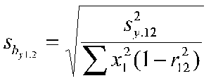
The standard error of the b weight with 2 IVs

This is the square root of the mean square residual over the sum of squares X₁ times 1 minus the squared correlation between IVs.

The sampling variance of the b weight with 2 IVs:

Notice the term on the far right.

The standard error of the b weight with multiple IVs:

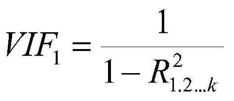
The term on the bottom right is the squared correlation where IV 1 is considered as a DV and all the other IVs are treated as IVs. The R-square term tells us how predcictable our IV is from the set of other IVs. It tells us about the linear dependence of one IV on all the other IVs.

The VIF for variable b1:

The VIF for variable i:

Big values of VIF are trouble. Some say look for values of 10 or larger, but there is no certain number that spells death. The VIF is also equal to the diagonal element of

R^-1, the inverse of the correlation matrix of IVs. Recall that

b =R^-1r, so we need to find R^-1 to find the beta weights.

This is easiest to see with a 2x2 matrix:

The determinant of R is |R| = (1)(1)-(r₁₂)(r₂₁) = 1 - r²₁₂. To find the inverse, we have to interchange main diagonal elements, reverse the sign of the off-diagonal elements, and divide each element by the determinant, like this:

As you can see, when r²₁₂ is large, VIF will be large.

When R is of order greater than 2 x 2, the main diagonal elements of R are 1/ R²_i, so we have the multiple correlation of the X with the other IVs instead of the simple correlation.

Small values of tolerance (close to zero) are trouble. Some computer programs will complain to you about tolerance. Do not interpret such complaints as computerized comments on silicon diversity; rather look to problems in collinearity.

Most multivariate statistical approaches (factor analysis, MANOVA, cannonical correlation, etc.) involve decomposing a correlation matrix into linear combinations of variables. The linear combinations are chosen so that the first combination has the largest possible variance (subject to some restrictions we won't discuss), the second combination has the next largest variance, subject to being uncorrelated with the first, the third has the largest possible variance, subject to being uncorrelated with the first and second, and so forth. The variance of each of these linear combinations is called an eigenvalue. You will learn about the kinds of decompositions and their uses in a course on multivariate statistics. We will only be using the eigenvalue for diagnosing collinearity in multiple regression.

SAS will produce a table for you that looks kind of like this (if you have 3 IVs): (Pedhazur, p. 303):

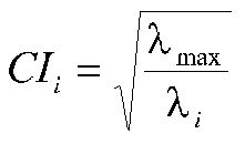
Number stands for linear combination of X variables. Eigenval(ue) stands for the variance of that combination. The condition index is a simple function of the eigenvalues, namely,

where l is the conventional symbol for an eigenvalue.

To use the table, you first look at the variance proportions. For X1, for example, most of the variance (about 75 percent) is associated with Number 3, which has an eigenvalue of .079 and a condition index of 6.90. Most of the rest of X1 is associated with Number 4. Variable X2 is associated with 3 different numbers (2, 3, & 4), and X3 is mostly associated with Number 2. Look for variance proportions about .50 and larger. Collinearity is spotted by finding 2 or more variables that have large proportions of variance (.50 or more) that correspond to large condition indices. A rule of thumb is to label as large those condition indices in the range of 30 or larger. There is no evident problem with collinearity in the above example. There is thought be a problem indicated in the example below (Pedhazur, p. 303):

The last condition index (15.128) is highly associated with X2 and X3. The b weights for X2 and X3 are probably not well estimated.

As you may have noticed, there are rules of thumb in deciding whether collinearity is a problem. People like to conclude that collinearity is not a problem. However, you should at least check to see if it seems to be a problem with your data. If it is, then you have some choices:

1. Lump it, but cautiously. Admit that there is ambiguity in the interpretation of the regression coefficients because they are not well estimated. Examine both the regression weights and zero order correlations together to see whether the results make sense. If the regression weights don't make sense, say so and refer to the correlation coefficients. Nonsignificant regression coefficients that correspond to "important" variables are very likely.
2. Select or combine variables. If you have multiple indicators of the same variable (e.g., two omnibus cognitive ability tests, two tests of conscientiousness, etc.), add them together (for an alternative, see point 3). If you are in a prediction only context, you may wish to use one of the variable selection methods (e.g., all possible regressions) to choose a useful subset of variables for your equation.
3. Factor analyze your IVs to find sets of relatively homogeneous IVs that you can combine (add together).
4. Use another type of analysis (path analysis, SEM).
5. Use another type of regression (ridge regression).
6. Try unit weights, that is, standardize each IV and then add them without estimating regression weights. Of course, this is no longer regression.