Write the regression equation for predicting Y from X in z-scores. Describe each term and say what the regression equation means.

Describe a concrete example (provide both words and numbers) in which two different groups could have the same correlation but different raw score b weights.

Describe a concrete example (provide both words and numbers) in which two different groups could have the same raw score b weights but different correlations.

Describe the sampling distribution of r. What are the main things that influence the shape and variance of this distribution?

Describe the sampling distribution of the regression line. What implication does this distribution have for the accuracy of predicted values of Y?

You have been introduced to both correlation and regression. You are now in a better position to appreciate how they are similar and different. In this section, I want to accomplish four things:

(1) review the connection between correlation and regression, presenting a geometric interpretation of correlation based on regression,

(2) revisit r and b in z score form,

(3) show how you can have different vales of r but the same slope (and vice versa), and

(4) talk about when you might prefer r to b or vice versa.

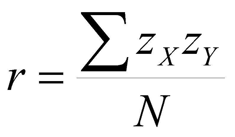
We have discussed the algebraic interpretation of r, that is,

which tells us the average of the z-score cross products. When we compute a regression equation, we regress Y on X to make our best predictions. We can also regress X on Y to predict values of X from values of Y. If we do so, the regression lines will only be the same if there is no error of prediction, that is, if and only if r = 1. Otherwise, there will be two distinct lines. If r = 0, then the two lines will be the respective means of Y and X, and the regression lines will be the same as the major axes of the figure. For values of r between 0 and 1, there will be two regression lines that form an interior angle less than 90 degrees, as illustrated in the figure below. The size of the interior angle is related to r.

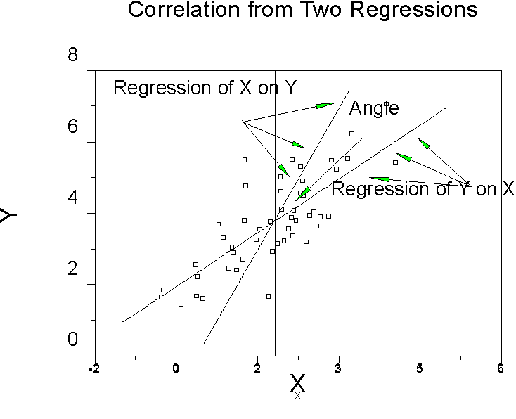
So the geometric interpretation of r is the size of the angle between the regression of y on x and of x on y. The smaller the angle, the larger the r.

If we make predictions in z scores instead of observed scores, we have

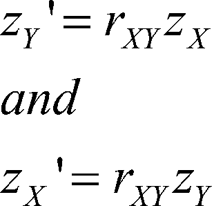
This says that the predicted value of X or Y in z-scores is just the predictor times r. The means of both variables are zero, so a is zero and drops out of the equation. Of course b equals r when X and Y are measured in z scores. The predicted value for Y measured as a z score is .

If we work with z_y for a moment, we have

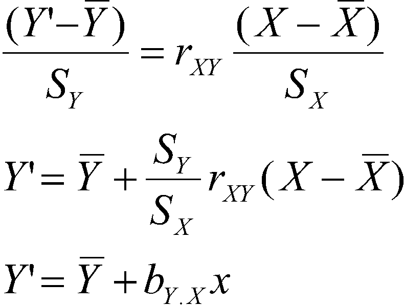
where

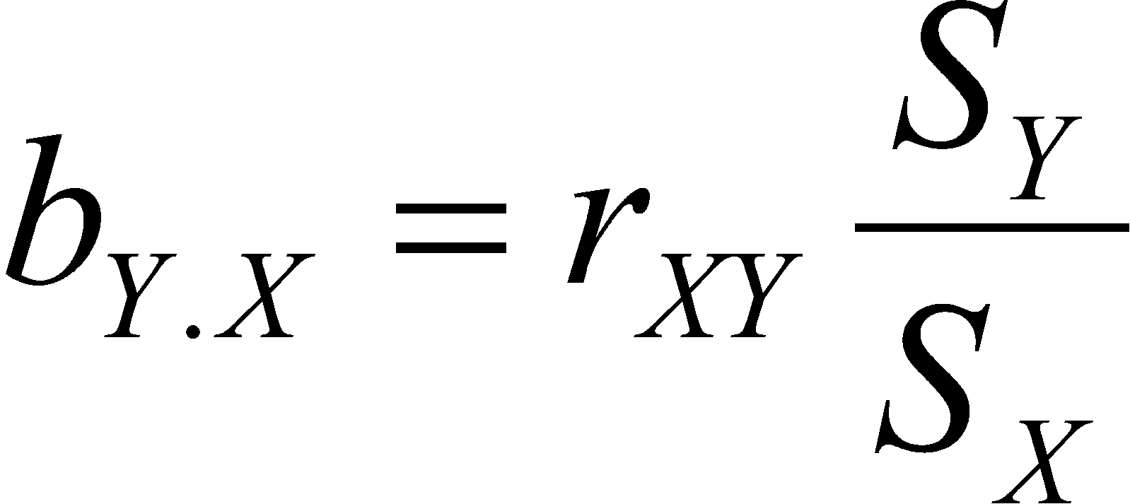
(You have already seen this equation once before. It is an example of the linear model where we have the grand mean of Y and an effect for X).

We can do the same for the regression of X on Y and if we do, we find that

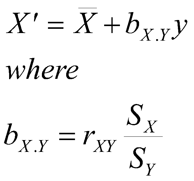
Therefore, it follows that the product of the two slopes equals r-squared, and that the harmonic mean of the two slopes is r.

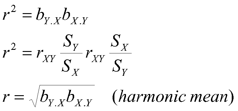
This is another way of saying that r and b are related; r is the harmonic mean of the two regression slopes and r-square is the product of the two slopes.

Some people find that describing the various relations between r and b is helpful in understanding them. Others find it more helpful to memorize a simple formula or two.

One more time: the correlation is the slope when both variables are measured as z scores (that is, when both X and Y are measured as z scores, r = b. For raw scores, we have

You can see that b and r will be equal whenever the ratio of the two standard deviations is 1.0. When S_Y is larger than S_X, the ratio will be greater than 1, and b will be larger than r. When S_X is larger than S_Y, the ratio will be less than 1.0, and b will be smaller than r.

You already know how to test for differences between values of r. For example, you could test whether the correlation between SAT and GPA is larger for males than for females. Soon you will be able to test for differences in b across groups. For example, you might test whether the regression slope for predicting GPA from SAT the same for males and females. Notice that the two tests will only mean the same thing if the ratio S_Y /S_X is the same for both males and females. It could be, for example, that the correlation for females is .60, S_Y for females is 1, and S_X for females 100. Then b would be .60(1/100) = .006. Now for males it could be that the correlation is .30, S_Y is 1, and S_X is 50. Then b is also .006 = .30(1/50). In this case, the correlation is quite different across groups (.60 vs. .30), but the slope is the same.

It is also possible to have the same correlation across groups, but have different slopes. Suppose that the correlation for both males and females is .60. Again suppose that for females is S_Y 1, and S_X for females 100. Then b for females would be .006. Now for males, suppose again that S_Y is 1, and S_X is 50. Then b for males is .012, which is twice that for females.

There are articles written about the difference in meaning between r and b. But what you just saw is all there is to know. They (b and r) are the same except for the ratio of standard deviations. Always report the correlation matrices (including means and standard deviations) whenever you do tests of either correlations or regressions. That way all the information is available and your reader can calculate either r or b if they don't like your choice.

 The Choice Between r and b

Most people choose to report correlations when they are estimating the associations between variables, especially when they are estimating the association between two variables as opposed to more than two. Because the correlation is the slope of z scores, it is comparable across settings and variables. If we see an r of .80, we know that there is a strong association regardless of the variables. Conversely, if we see an r of .18, we know the association is a weak one. We often use correlations when we want to compare the strength of association from one setting to another or from one variable to another.

Most people report regressions when they are making predictions of one variable from another (that is, point predictions). For example, if we wanted to predict GPA from SAT scores, we would probably report one or more regression equations. If our equation is GPA = 1+.0035SAT, then we can output a predicted GPA for any SAT score (if SAT =800, then GPA is predicted to be 3.8, if 500 then 2.75, and if 200, then 1.7 and so forth). We often use regression for applied prediction problems.

Other than purpose, the key to meaningful regression estimates is the meaning of units of measurement in our variables. The intercept has meaning only when the value of X=0 has meaning. With the SAT for a predictor, the intercept has no meaningful interpretation (the lowest possible score on an SAT scale is 200). Whether the slope has meaning depends upon the meaning of the units of Y. With the prediction of GPA, knowing that when SAT changes one unit, GPA changes .0035 units says something. Perhaps it would be better to say that GPA changes .35 points when SAT changes 100 points, so that a change from an SAT of 800 to 700 results in an expected change in GPA from 3.8 to 3.45. So the slope is informative if our Y units mean something to us. If we are talking about two questionnaires or clinical scales then the units of Y refer mainly to marks on a piece of paper and the slope has little meaning. For example consider the regression of a measure of job satisfaction on a measure of job challenge or consider the regression of an MMPI scale on the Beck Depression Inventory. In both these cases, the slope won't be terribly meaningful, and r might be a better choice for reporting.

The sampling distribution of the correlation depends upon r and N. Let's look at a couple of empirical sampling distributions.

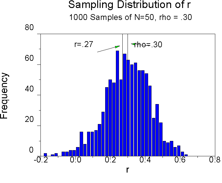
Note that the distribution is a little skewed, as it will be when r is not zero. The mean of this distribution is .295, so r is a pretty good estimate of r on average, even if it is a little biased. Also note that only a few correlations are less than zero in the distribution. The big problem here is that the samples are of size 50. The critical value of r for that sample size is .27. If he correlation is about .27 or larger, we will conclude that it is significant, that is, we will conclude it was drawn from a population where r is not zero. But in our case, we will be mistaken about half of the time. About half of the correlations we observe when r = .30 and our sample size is 50 fall below r = .27. This is a power problem. We will falsely conclude that r =0 about half of the time we did such a study. Small population correlations are all too frequent. Use large samples whenever you can.

Let's look at a sampling distribution given r = .80.

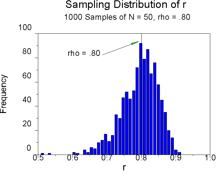
As you can see, the sampling distribution is somewhat more skewed. However, the mean of this distribution is .795, which also indicates minimal bias. None of the 1,000 correlations drawn from this population are even close to the .27 critical value, so power is not a problem here. If the population correlation is .8 and you have a sample size of 50, you will be able to reject the null. Of course, it's unusual to have correlations of this magnitude except when comparing measures of the same thing (e.g., test-retest, alternate forms, etc.).

Let's look at the sampling distribution of a regression line.

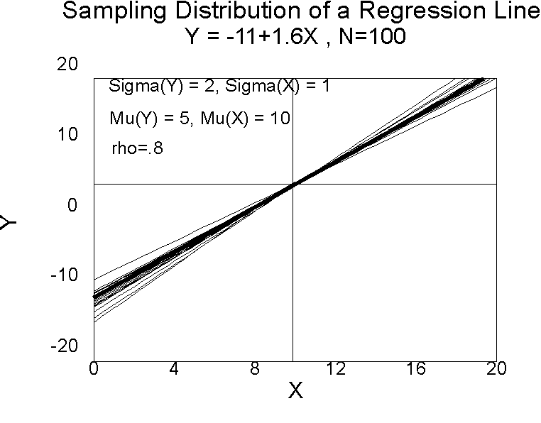
Note the fan shape. When we take samples from a population, the means of X and Y will tend to be close to their population mean. The regression line always passes through the means of X and Y, so each regression line will pass close to the middle of the graph. Differences in the slope for the same means (same 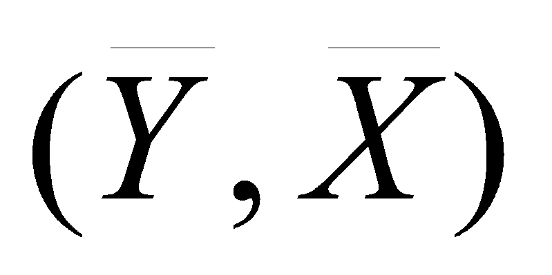pairs) produce a fan shape that becomes increasingly wide as the distance from the means increases. The confidence interval around the regression line becomes increasingly wide as the distance from the mean increases because variance of lines in the sampling distribution about the population line increases as the distance from the means increases. Because of this fan shape, confidence intervals for values of Y' farther from the mean are broader than are confidence intervals for values of Y' closer to the mean.