What is the logistic curve? What is the base of the natural logarithm? Why do statisticians prefer logistic regression to ordinary linear regression when the DV is binary? How are probabilities, odds and logits related? What is an odds ratio? How can logistic regression be considered a linear regression? What is a loss function? What is a maximum likelihood estimate? How is the b weight in logistic regression for a categorical variable related to the odds ratio of its constituent categories?

This chapter is difficult because there are many new concepts in it. Studying this may bring back feelings that you had in the first third of the course, when there were many new concepts each week.

For this chapter only, we are going to deal with a dependent variable that is binary (a categorical variable that has two values such as "yes" and "no") rather than continuous.

[Technical note: Logistic regression can also be applied to ordered categories (ordinal data), that is, variables with more than two ordered categories, such as what you find in many surveys. However, we won't be dealing with that in this course and you probably will never be taught it. If our dependent variable has several unordered categories (e.g., suppose our DV was state of origin in the U.S.), then we can use something called discriminant analysis, which will be taught to you in a course on multivariate statistics.]

It is customary to code a binary DV either 0 or 1. For example, we might code a successfully kicked field goal as 1 and a missed field goal as 0 or we might code yes as 1 and no as 0 or admitted as 1 and rejected as 0 or Cherry Garcia flavor ice cream as 1 and all other flavors as zero. If we code like this, then the mean of the distribution is equal to the proportion of 1s in the distribution. For example if there are 100 people in the distribution and 30 of them are coded 1, then the mean of the distribution is .30, which is the proportion of 1s. The mean of the distribution is also the probability of drawing a person labeled as 1 at random from the distribution. That is, if we grab a person at random from our sample of 100 that I just described, the probability that the person will be a 1 is .30. Therefore, proportion and probability of 1 are the same in such cases. The mean of a binary distribution so coded is denoted as P, the proportion of 1s. The proportion of zeros is (1-P), which is sometimes denoted as Q. The variance of such a distribution is PQ, and the standard deviation is Sqrt(PQ). {Why can't all of stats be this easy?}

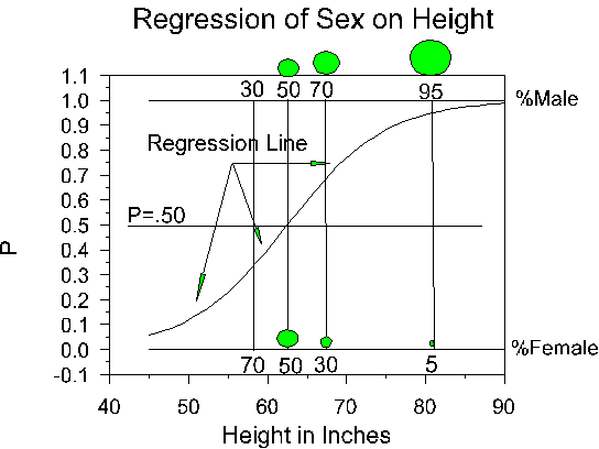
Suppose we want to predict whether someone is male or female (DV, M=1, F=0) using height in inches (IV). We could plot the relations between the two variables as we customarily do in regression. The plot might look something like this:

Points to notice about the graph (data are fictional):

1. The regression line is a rolling average, just as in linear regression. The Y-axis is P, which indicates the proportion of 1s at any given value of height. (review graph)
2. The regression line is nonlinear. (review graph)
3. None of the observations --the raw data points-- actually fall on the regression line. They all fall on zero or one. (review graph)

When I was in graduate school, people didn't use logistic regression with a binary DV. They just used ordinary linear regression instead. Statisticians won the day, however, and now most psychologists use logistic regression with a binary DV for the following reasons:

1. If you use linear regression, the predicted values will become greater than one and less than zero if you move far enough on the X-axis. Such values are theoretically inadmissible.
2. One of the assumptions of regression is that the variance of Y is constant across values of X (homoscedasticity). This cannot be the case with a binary variable, because the variance is PQ. When 50 percent of the people are 1s, then the variance is .25, its maximum value. As we move to more extreme values, the variance decreases. When P=.10, the variance is .1*.9 = .09, so as P approaches 1 or zero, the variance approaches zero.
3. The significance testing of the b weights rest upon the assumption that errors of prediction (Y-Y') are normally distributed. Because Y only takes the values 0 and 1, this assumption is pretty hard to justify, even approximately. Therefore, the tests of the regression weights are suspect if you use linear regression with a binary DV.

The logistic curve relates the independent variable, X, to the rolling mean of the DV, P (). The formula to do so may be written either

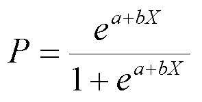
Or

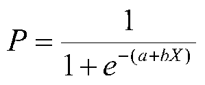
where P is the probability of a 1 (the proportion of 1s, the mean of Y), e is the base of the natural logarithm (about 2.718) and a and b are the parameters of the model. The value of a yields P when X is zero, and b adjusts how quickly the probability changes with changing X a single unit (we can have standardized and unstandardized b weights in logistic regression, just as in ordinary linear regression). Because the relation between X and P is nonlinear, b does not have a straightforward interpretation in this model as it does in ordinary linear regression.

A loss function is a measure of fit between a mathematical model of data and the actual data. We choose the parameters of our model to minimize the badness-of-fit or to maximize the goodness-of-fit of the model to the data. With least squares (the only loss function we have used thus far), we minimize SS_res, the sum of squares residual. This also happens to maximize SS_reg, the sum of squares due to regression. With linear or curvilinear models, there is a mathematical solution to the problem that will minimize the sum of squares, that is,

Or

With some models, like the logistic curve, there is no mathematical solution that will produce least squares estimates of the parameters. For many of these models, the loss function chosen is called maximum likelihood. A likelihood is a conditional probability (e.g., P(Y|X), the probability of Y given X). We can pick the parameters of the model (a and b of the logistic curve) at random or by trial-and-error and then compute the likelihood of the data given those parameters (actually, we do better than trail-and-error, but not perfectly). We will choose as our parameters, those that result in the greatest likelihood computed. The estimates are called maximum likelihood because the parameters are chosen to maximize the likelihood (conditional probability of the data given parameter estimates) of the sample data. The techniques actually employed to find the maximum likelihood estimates fall under the general label numerical analysis. There are several methods of numerical analysis, but they all follow a similar series of steps. First, the computer picks some initial estimates of the parameters. Then it will compute the likelihood of the data given these parameter estimates. Then it will improve the parameter estimates slightly and recalculate the likelihood of the data. It will do this forever until we tell it to stop, which we usually do when the parameter estimates do not change much (usually a change .01 or .001 is small enough to tell the computer to stop). [Sometimes we tell the computer to stop after a certain number of tries or iterations, e.g., 20 or 250. This usually indicates a problem in estimation.]

Suppose we only know a person's height and we want to predict whether that person is male or female. We can talk about the probability of being male or female, or we can talk about the odds of being male or female. Let's say that the probability of being male at a given height is .90. Then the odds of being male would be

.

(Odds can also be found by counting the number of people in each group and dividing one number by the other. Clearly, the probability is not the same as the odds.) In our example, the odds would be .90/.10 or 9 to one. Now the odds of being female would be .10/.90 or 1/9 or .11. This asymmetry is unappealing, because the odds of being a male should be the opposite of the odds of being a female. We can take care of this asymmetry though the natural logarithm, ln. The natural log of 9 is 2.217 (ln(.9/.1)=2.217). The natural log of 1/9 is -2.217 (ln(.1/.9)=-2.217), so the log odds of being male is exactly opposite to the log odds of being female. The natural log function looks like this:

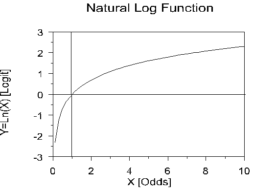
Note that the natural log is zero when X is 1. When X is larger than one, the log curves up slowly. When X is less than one, the natural log is less than zero, and decreases rapidly as X approaches zero. When P = .50, the odds are .50/.50 or 1, and ln(1) =0. If P is greater than .50, ln(P/(1-P) is positive; if P is less than .50, ln(odds) is negative. [A number taken to a negative power is one divided by that number, e.g. e^-10 = 1/e^10. A logarithm is an exponent from a given base, for example ln(e¹⁰) = 10.]

Back to logistic regression.

In logistic regression, the dependent variable is a logit, which is the natural log of the odds, that is,

So a logit is a log of odds and odds are a function of P, the probability of a 1. In logistic regression, we find

logit(P) = a + bX,

Which is assumed to be linear, that is, the log odds (logit) is assumed to be linearly related to X, our IV. So there's an ordinary regression hidden in there. We could in theory do ordinary regression with logits as our DV, but of course, we don't have logits in there, we have 1s and 0s. Then, too, people have a hard time understanding logits. We could talk about odds instead. Of course, people like to talk about probabilities more than odds. To get there (from logits to probabilities), we first have to take the log out of both sides of the equation. Then we have to convert odds to a simple probability:

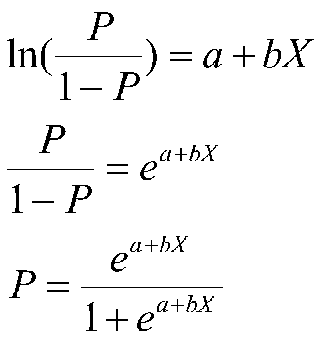
The simple probability is this ugly equation that you saw earlier. If log odds are linearly related to X, then the relation between X and P is nonlinear, and has the form of the S-shaped curve you saw in the graph and the function form (equation) shown immediately above.

Suppose that we are working with some doctors on heart attack patients. The dependent variable is whether the patient has had a second heart attack within 1 year (yes = 1). We have two independent variables, one is whether the patient completed a treatment consistent of anger control practices (yes=1). The other IV is a score on a trait anxiety scale (a higher score means more anxious).

 Our data:

  Our correlation matrix:

Note that half of our patients have had a second heart attack. Knowing nothing else about a patient, and following the best in current medical practice, we would flip a coin to predict whether they will have a second attack within 1 year. According to our correlation coefficients, those in the anger treatment group are less likely to have another attack, but the result is not significant. Greater anxiety is associated with a higher probability of another attack, and the result is significant (according to r).

Now let's look at the logistic regression, for the moment examining the treatment of anger by itself, ignoring the anxiety test scores. SAS prints this:

SAS tells us what it understands us to model, including the name of the DV, and its distribution.

Then we calculate probabilities with and without including the treatment variable.

 The computer calculates the likelihood of the data. Because there are equal numbers of people in the two groups, the probability of group membership initially (without considering anger treatment) is .50 for each person. Because the people are independent, the probability of the entire set of people is .50²⁰, a very small number. Because the number is so small, it is customary to first take the natural log of the probability and then multiply the result by -2. The latter step makes the result positive. The statistic -2LogL (minus 2 times the log of the likelihood) is a badness-of-fit indicator, that is, large numbers mean poor fit of the model to the data. SAS prints the result as -2 LOG L. For the initial model (intercept only), our result is the value 27.726. This is a baseline number indicating model fit. This number has no direct analog in linear regression. It is roughly analogous to generating some random numbers and finding R² for these numbers as a baseline measure of fit in ordinary linear regression. By including a term for treatment, the loss function reduces to 25.878, a difference of 1.848, shown in the chi-square column. The difference between the two values of -2LogL is known as the likelihood ratio test.

When taken from large samples, the difference between two values of -2LogL is distributed as chi-square:

Recall that multiplying numbers is equivalent to adding exponents (same for subtraction and division of logs).

This says that the (-2Log L) for a restricted (smaller) model - (-2LogL) for a full (larger) model is the same as the log of the ratio of two likelihoods, which is distributed as chi-square. The full or larger model has all the parameters of interest in it. The restricted is said to be nested in the larger model. The restricted model has one or more of parameters in the full model restricted to some value (usually zero). The parameters in the nested model must be a proper subset of the parameters in the full model. For example, suppose we have two IVs, one categorical and once continuous, and we are looking at an ATI design. A full model could have included terms for the continuous variable, the categorical variable and their interaction (3 terms). Restricted models could delete the interaction or one or more main effects (e.g., we could have a model with only the categorical variable). A nested model cannot have as a single IV, some other categorical or continuous variable not contained in the full model. If it does, then it is no longer nested, and we cannot compare the two values of -2LogL to get a chi-square value. The chi-square is used to statistically test whether including a variable reduces badness-of-fit measure. This is analogous to producing an increment in R-square in hierarchical regression. If chi-square is significant, the variable is considered to be a significant predictor in the equation, analogous to the significance of the b weight in simultaneous regression.

For our example with anger treatment only, SAS produces the following:

The intercept is the value of a, in this case -.5596. As usual, we are not terribly interested in whether a is equal to zero. The value of b given for Anger Treatment is 1.2528. the chi-square associated with this b is not significant, just as the chi-square for covariates was not significant. Therefore we cannot reject the hypothesis that b is zero in the population. Our equation can be written either:

Logit(P) = -.5596+1.2528X

Or

The main interpretation of logistic regression results is to find the significant predictors of Y. However, other things can sometimes be done with the results.

Recall that the odds for a group is :

Now the odds for another group would also be P/(1-P) for that group. Suppose we arrange our data in the following way:

Now we can compute the odds of having a heart attack for the treatment group and the no treatment group. For the treatment group, the odds are 3/6 = 1/2. The probability of a heart attack is 3/(3+6) = 3/9 = .33. The odds from this probability are .33/(1-.33) = .33/.66 = 1/2. The odds for the no treatment group are 7/4 or 1.75. The odds ratio is calculated to compare the odds across groups.

If the odds are the same across groups, the odds ratio (OR) will be 1.0. If not, the OR will be larger or smaller than one. People like to see the ratio be phrased in the larger direction. In our case, this would be 1.75/.5 or 1.75*2 = 3.50.

Now if we go back up to the last column of the printout where is says odds ratio in the treatment column, you will see that the odds ratio is 3.50, which is what we got by finding the odds ratio for the odds from the two treatment conditions. It also happens that e^1.2528 = 3.50. Note that the exponent is our value of b for the logistic curve.