Give a concrete example (names of variables, context) in which it makes sense to compute a partial correlation. Why a partial rather than a semipartial?

Give a concrete example (names of variables, context) in which it makes sense to compute a semipartial correlation. Why a semipartial rather than a partial?

Why is the squared semipartial always less than or equal to the partial correlation?

Why is regression more closely related to the semipartial than the partial correlation?

Describe how you would go about computing a third order partial correlation.

Regression tends to be a lot more complicated and difficult than ANOVA. The difficulty comes because there are so many concepts in regression and correlation. The excessive number of concepts comes because the problems we tackle are so messy. With ANOVA, you assign people to treatments, and all sorts of explanations of the results (that is, the associations or correlations between the IVs and DV) get ruled out. With nonexperimental data, we cannot assign people to treatments for practical or ethical reasons. People are always interested in the difference between men & women but we really can't assign people to those groups.

We measure individual differences in many things, including cognitive ability, personality, interests & motives, attitudes, and so forth. Many times, we want to know about the influence of one IV on a DV, but one or more other IVs pose an alternative explanation. We would like to hold some third variable constant while examining the relations between X and Y. With assignment we can do this by design. With measures of individual differences, we can do this statistically rather than by manipulation.

The basic idea in partial and semipartial correlation is to examine the correlations among residuals (errors of prediction). If we regress variable X on variable Z, then subtract X' from X, we have a residual e. This e will be uncorrelated with Z, so any correlation X shares with another variable Y cannot be due to Z.

 Example

There is at present a debate among educators and policy makers about the use of aptitude and achievement tests as part of college admissions. Some say aptitude tests should be used because they are minimally influenced by formal education. Thus, they tend to level the playing field and account for differences among schools in grade inflation. Other say that achievement tests should be used because they show what people actually know or can do, and they would provide motivation for students to progress beyond basics. There are many complicated arguments that have some merit on both sides. Let's set all that to one side for a moment and think about the utility of such measures for a moment. Suppose what we want to do is to make good admissions decisions in the sense that we want to maximize our prediction of achievement in college from what we know from the end of high school in the area of mathematics. Suppose admit people to college without looking at the data, which are test scores for people on the SAT-Q (quantitative or math aptitude), and scores on a math CLEP test (math achievement) and we look at grades in the standard first year math sequence (differential and integral calculus). We want to know about the prediction of math grades from the two tests.

Our data might look like this:

The correlations among our three variables are as follows:

Clearly, both our tests are related to college math mastery as indicated by GPA.

Suppose we regress GPA on SAT-Q. Our regression equation is GPA' = 1.78+.002SATQ and R-square is .52.

If we print our variables, predicted values and residuals, we get:

If we compute the correlations among these variables, we find

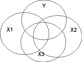
Note that SAT and GPA are still correlated .72. SAT and PRED are correlated 1.0. After all, PRED is a linear function of SAT (i.e., a linear transformation of the form Y'=1.78+.002SAT). Especially note that RESID is uncorrelated with SATQ, that is, the correlation between PRED and RESID is zero. Of course, the correlation of SAT and RESID is also zero. Remember that the linear model says that the variance in Y is due in part to X and in part to error. The part due to X is a linear function of X that is perfectly correlated with X. What ever is left (the residual) is what is left when the part due to X is subtracted out. Therefore, the residual must be uncorrelated with X. Recall your Venn Diagrams. Just because the residual is uncorrelated with X doesn't mean it cannot correlated with other things. Note that the residual is correlated .69 with GPA. In our case, you might say that the residual is that part of GPA which is left when SAT is taken out. OK, go ahead and say it!

Now we could also do the same thing predicting GPA from math achievement, our CLEP score. If we do that, we find that GPA'=1.17+.06CLEP and R-square =.77. The correlations among these variables are:

Note that the correlation between CLEP and GPA is larger than for SAT and GPA. Also note that the correlation between the residual and GPA is smaller. But again the predicted values correlate perfectly with the IV and the residuals do not correlate with the IV or predicted values.

One other thing that we could do help determine a pragmatic argument is to regress GPA on both SAT and CLEP at the same time to see what happens. If we do that, we find that R-square for the model is .78, F = 12.25, p < .01. The intercept and b weight for CLEP are both significant, but the b weight for SAT is not significant. The values are

Intercept = 1.16, t=2.844, p < .05

CLEP = 0.07, t=2.874, p < .05

SATQ = -.0007, t=-0.558, n.s.

In this case, we would conclude that the significant unique predictor is CLEP. Although SAT is highly correlated with GPA, it adds nothing to the prediction equation once the CLEP score is entered. (These data are fictional and the sample size is much too small to run this analysis. It's there for illustration only.)

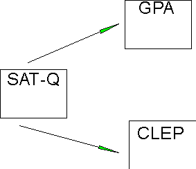
Now suppose we wanted to argue something a little different. Suppose we had a theory that said that all measures of math achievement share a common explanation, which is math ability. In other words, the reason that various (all) math achievement tests are correlated is that they share the math ability factor. In other words, math ability explains the correlation between achievement tests. In path diagram form, we might represent this something like this:

Now it may not be immediately obvious, but this diagram says that there is only one common cause of GPA and CLEP, which is SATQ. This implies that the correlation between GPA and CLEP is due solely to SATQ. If there were other theoretical explanations (e.g., motivation), then these should be drawn into the diagram. As it is, this says that the correlation between GPA and CLEP would be zero except for the shared influence of SATQ.

We have already found the residual of GPA when we regressed GPA on SATQ. We know that this residual is not correlated with SATQ. We can run another regression where we predict CLEP from SATQ. If we do this, we find that CLEP' = 8.57+.04SATQ. R-square is .76. We can also see the values of the variables:

  The correlations among these variables are

Note that the residuals are not correlated with SAT. Now we have two sets of residuals from SAT, one for GPA and one for CLEP. GPA and CLEP are our two achievement measures. According to our theory, they should not be correlated except for the common influence of SAT. The residuals are what is left when we remove SAT from each variable. Therefore, our theory says that our two residuals should not be correlated.

If we compute the correlation between these two sets of residual, we find that:

The correlation between the two sets is .73, which is significantly different from zero at p < .05. Thus we can reject our hypothesis that the correlation between GPA and CLEP is explained solely by SAT. Taking it a step further, we may seriously question the theory that the only common cause of the two achievement indices is math ability. Of course, there are always other explanations (our SAT is bad measure of ability? something strange about the sample? the courses that went into the computation of GPA, etc.).

The correlation between the two sets of residuals is called a partial correlation. In our case, it was the correlation between GPA and CLEP while holding SAT constant.

The partial correlation is what we get when we hold constant some third variable from two other variables. We know the correlation between CLEP and GPA is .88. But SAT "accounts for" (or could account for) part of that. What would happen to the correlation if SAT-Q were constant? It is .73, the correlation of the residuals from predicting CLEP and GPA from SATQ.

There are many substantive areas in psychology were we want to know partial correlations (Name 1?).

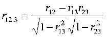
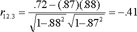
Pedhazur denotes the partial correlation r_12.3 where r₁₂ is the correlation between X₁ and X₂ and the _.3 means the partial controlling for X₃. In our example, it is the correlation between GPA and CLEP while holding SATQ constant.

The formula to compute the partial r from correlations is

In our example, (1 = GPA, 2 = CLEP, 3 = SAT)

You won't be using this equation to figure partials very often, but it's important for two reasons: (1) the partial correlation can be (a little or a lot) larger or smaller then the simple correlation, depending on the signs and size of the correlations used, and (2) for its relation to the semipartial correlation.

If we partial one variable out of a correlation, that partial correlation is called a first order partial correlation. If we partial out 2 variables from that correlation (e.g., r_12.34), we have a second order partial, and so forth. It is customary to refer to unpartialed (raw, as it were) correlations as zero order correlations. We can use formulas to compute second and higher order partials, or we can use multiple regression to compute residuals. For example, we could regress each of X₁ and X₂ on both X₃ and X₄ simultaneously and then compute the correlation between the residuals.

If we did that, we could be computing r_12.34, the correlation between X₁ and X₂, controlling for both X₃ and X₄.

We can compute partials from R². For example

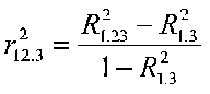
Of course we have some confusing terminology for you, but let's explore the meaning of this. This says that the squared first order partial (the partial of 1 and 2 holding 3 constant) is equal to the difference between two R² terms divided by 1 minus an R² term. The first R² term is R²_1.23, which is the squared multiple correlation when X₁ is the DV and X₂ and X₃ are the IVs (this is not a partial, it just looks that way to be confusing). The second R² is R²_1.3, which is the squared correlation when X₁ is the DV and X₃ is the IV. This is also the term that appears in the denominator.

When we add IVs to a regression equation (first include them), R² either stays the same or increases. If the new variable adds to the prediction of the DV, then R² increases. If the new variable adds nothing, R² stays the same.

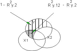
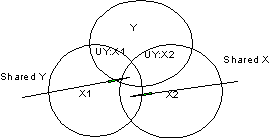
In Figure A, the R² for X₁ will be the overlapping portion Y and X₁ in the figure. When we add X₂ to the equation, R² will increase by the part of Y that overlaps with X₂. Because X₁ and X₂ are orthogonal, R² for the model with both X₁ and X₂ will be r²_y1 + r²_y2. In Figure B, when we put X₁ into the regression equation, the R² will be the overlapping portion with Y, that is, R²_y.1 is UY: X₁+Shared Y. When we add X₂ to the equation, R²_y.12 will be the total overlapping portion of Y with both X variables, that is, R² will be UY: X₁ + Shared Y + UY: X₂. The increase in R² that we see when we add X₂ if X₁ is already in the equation will be UY: X₂.

Suppose we start over. We start with X₂ in the regression equation. Then R²_y.2 will be UY: X₂ + Shared Y. If we then add X₁ to the equation, R² will increase to UY: X₂ + Shared Y + UY: X₁. In both cases the shared Y is counted only once and it shows up the first time any variable that shares it is included in the model. In Figure C, the variables overlap little, and the addition of each X variable into the equation increases R². In Figure D, X₃ overlaps completely with X₁ and X₂. If we add X₃ after X₁ and X₂, R² will not increase. However, adding variables never causes R² to decrease (look at the figures).

Now back to the equation:

(I've changed symbols slightly to match the figures.) The term on the left is a squared correlation (a shared variance). On the right in the numerator is a difference between two R² terms. It is actually an increment in R². It shows the increase in R² when we move from predicting Y from X₂ (right term) to predicting Y from X₁ and X₂ (left term). Because R² never decreases, R²_y.12 will always be greater than or equal to R²_y.2. The difference in R² will be UY: X₁, that is, the R² due to X₁ above and beyond that due to X₂. The numerator is the shared variance of Y unique to X₁ (UY: X₁). So we have partialed out X₂ from X₁ on top. But we still have to remove the influence of X₂ from Y, and this is done in the denominator, where we subtract R²_Y.2 from 1.

The squared correlation is the percentage of shared variance (r²_Y1.2). In figure B, the squared partial correlation of X₁ with Y controlling for X₂ will be UY: X₁/[Total Y-(UY: X₂+Shared Y)]. Note how X₂ is removed both from X₁ and from Y.

With partial correlation, we find the correlation between X and Y holding Z constant for both X and Y. Sometimes, however, we want to hold Z constant for just X or just Y. In that case, we compute a semipartial correlation. A partial correlation is computed between two residuals. A semipartial is computed between one residual and another raw or unresidualized variable. The notation r_1(2.3) means the semipartial correlation between unmodified X₁ and residualized X₂, where X₃ has been taken from X₂.

Let's compare the correlational formulas for the partial and semipartial--

Partial:

Semipartial

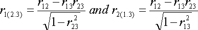
Note that the partial and semipartial correlation formulas are the same in the numerator and almost the same in the denominator. The partial contains something extra, that is, something missing from the semipartial correlation in the denominator. This means that the partial correlation is going to be larger in absolute value than the semipartial. This will be true except when the controlling or partialling variable is uncorrelated with the variable to be controlled or residualized; this is a trivial case.

Back to our educational debate. Suppose we want to predict college math grades. Someone argues that once we know CLEP (advanced achievement in math) scores, there is no need to know SATQ. SATQ will add nothing to the prediction of GPA once we know CLEP, says the argument. In this case we will want to partial CLEP from SAT, but not from GPA. That is, we hold CLEP constant for the SAT, and see whether the SAT so residualized can still predict GPA.

In our example, (1 = GPA, 2 = SAT, 3 = CLEP)

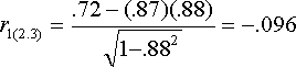
The correlation between GPA and SAT taking CLEP from SAT is -.096. This corresponds to the scenario of interest. It shows that there is basically no correlation between SAT and GPA when we hold CLEP constant. The other formula for the semipartial shows what happens if we partial CLEP from GPA but not SAT. This partial is shown below. It is not really of interest in the current case, but is presented anyway for completeness of computational examples.

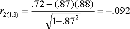
If we partial the CLEP from both GPA and SAT, the correlation is:

The result doesn't make much intuitive sense, but it does remind us that the absolute value of the partial is larger than the semipartial.

One interpretation of the semipartial is that it is the correlation between one variable and the residual of another, so that the influence of a third variable is only paritialed from one of two variables (hence, semipartial). Another interpretation is that the semipartial shows the increment in correlation of one variable above and beyond another. This is seen most easily with the R² formulation.

Let's compare partial and semipartial squared correlations:

Partial

Semipartial

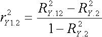
This says that the squared semipartial correlation is equal to the difference between two R² values. The difference between the squared partial and semipartial correlations is solely in the denominator. Note that in both formulas, the two R² values are incremental. That is, the left R² is the squared correlation when X₁ is the DV and X₂ and X₃ are IVs. The right R² is the squared correlation when X₁ is the DV and X₃ is the IV. The difference between the two values, of course, is due to X₂. The difference in R² is the incremental R² for variable X₂. In terms of our Venn diagrams, X₁ is Y, X₂ is X₁ and X₃ is X₂. Therefore, the squared semipartial correlation r²_y(1.2) is R²_y.12 - R²_y.2 or UY: X₁. The other semipartial would be R²_y.12 - R²_y.1.

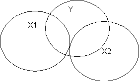
Both the squared partial and squared semipartial correlations indicate the proportion of shared variance between two variables. The partial tends to be larger than the semipartial. To see why, consider our familiar diagram:

The partial correlation of X₁ and Y controlling for X₂ considers the ratio of UY: X₁ to the part of Y that overlaps neither X variable, that is, UY: X₁ to [Y-(Shared Y+UY: X₂)]. This is because the partial removes X₂ from both X₁ and Y. The semipartial correlation between X₁ and Y r_y(1.2), however, corresponds the ratio of UY: X₁to all of Y. This is because X₂ is only taken from X₁, not from Y.

In our example,

Y = GPA = variable 1

X₁ = CLEP = variable 2; it's r with GPA was .8763, R-square is .7679.

X₂ = SAT = variable 3; its r with GPA was .7181; R-square was .5156.

R-square for GPA on both SAT and CLEP was .7778.

This agrees with our earlier estimate within rounding error, as .73*.73 = .53.

Earlier estimate:

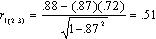
and .51*.51 = .26.

Regression is about semipartial correlations. For each X variable, we ask "What is the contribution of this X above and beyond the other X variables?" In essence, we regress each new X variable on the other X variables, and then correlate the residualized X with Y.

That would be a partial correlation, not a semipartial correlation. The change in R² that we get by including each new X variable in the regression equation is a squared semipartial correlation that corresponds to a b weight. The b weight provides a clue to answering the question "What is the correlation between {X residualized on the other X variables} and {Y}?" Another way of saying this is that the b weight tells us the slope of Y on this X while holding the other X variables in the regression equation constant.

Suppressor variables are a little hard to understand. I have 3 reasons to discuss them: (1) they prove that inspection of a correlation matrix is not sufficient to tell the value of a variable in a regression equation, (2) sometimes they happen to you, and you have to know what is happening to avoid making a fool of yourself, and (3) they show why Venn diagrams are sometimes inadequate for depicting multiple regression.

The operation of a suppressor is easier to understand if you first think of measured variables as composites (simple or weighted sums) of other variables.

For example, we get a total test score that is the total of the scores on the items of a test. Or we get a job satisfaction overall score that is the total of the facet satisfaction scores. Now suppose that a composite is made by adding two things together that are negatively correlated with one another. For example, suppose we want to know your total attraction to an automobile and we get this by getting your satisfaction with cars by summing your satisfaction with attributes such as price and prestige. So we ask you to rate a bunch of cars on the attributes and we sum them. Now if you like the prestige, you won't like the price, and vice versa. If we add these two things, we get a total satisfaction score, but it has to parts to it that are antagonistic (negatively correlated) across cars. Note that this could happen even if we never asked you for ratings of multiple attributes, but rather asked for your overall satisfaction. Observed measures can be composites of lots of things, some positively correlated, some negatively correlated, and some uncorrelated.

Suppose we have two independent variables; X₁ is correlated with the criterion, and X₂ is not (or nearly so), but it is correlated with the first. Suppose we collected sales performance data (dollars sold per month) for a series of professional sales people (Y). Suppose we ask supervisors for judgment of sales performance for each, that is, how much they like their sales performance (X₁). We also ask how much each supervisor likes each sales person as a person (X₂). We have collected some data on these three variables and find that the results can be summarized in the following correlation matrix:

Note that X₁ is correlated with Y. X₂ is not correlated with Y, but it is correlated with X₁. In this case, X₂ will be a suppressor. We can solve for beta weights by R^-1r = b.

Note that the beta weight for X₂ is negative although the correlation between X₂ and Y is zero. This can also happen sometimes when r for X₂ is (usually slightly) positive.

Note also that the beta weight for X₁ is positive, and actually larger than its corresponding r of .50. The R² for the two variable model is (.50)*(.667) or .334. This is larger than .50² or .25 that would have been guessed solely on the basis of X₁ (X₂ might have been disregarded because of its zero correlation with Y). How can this happen? Three ways to explain the suppressor variable.

1. X₂ is not correlated with Y, but X₁ is. X₁ is also correlated with X₂. The part of X₁ that is correlated with X₂ is of no use in predicting Y. If we residualize X₁ on X₂, X₁ will be better able to predict Y because we will have removed part of it that has nothing to do with Y. X₂ is a measure of prediction error in X₁. If we subtract X₂ (the negative b weight) from X₁, we will improve our prediction (increase the positive b weight for X₁). Because X₂ is a measure of error, it suppresses the correlation with Y, hence the term suppressor. This is, I think, the reasoning that caused the term.
2. X₁ and X₂ share something (r = .50) that is not related to Y. When we compute the semipartial correlations of each X with Y, we remove that common part. This makes the b weight increasingly positive for X₁ and negative for X₂. The reason the X₂ weight is negative is because the part of X₂ that is negatively related to Y is what is left over when we remove the part that is not related to Y; the removed part (taken through residualizing X₂) was masking the negative relations between X₂ and Y in the raw variables.
3. The beta weights are taken by finding the inverse of the matrix R and multiplying this by the observed correlations, r. (Although we're talking about beta weights, this applied equally to b weights.) Whenever we have positive correlations among our predictors, the inverse will have to contain negative elements to orthogonalize R. When these negative elements are multiplied by r, the observed correlations, the beta weights will become negative unless the observed correlations are strongly positive. This is a consequence of the positive correlations among the predictors. The suppressor is just a special case of what happens when you invert the predictor matrix in the usual case when independent variables are positively correlated.

Let's return to the three reasons for learning about suppressors. First, inspection of the correlation matrix may be insufficient to tell the value of a variable in a regression equation. It turns out that X₂ was a valuable contributor to predicting Y, and this would not have been obvious from simply looking at the correlations of each X with Y. With just two IVs, you can tell that suppression is likely because of the pattern of correlations. With larger numbers of variables, it becomes increasingly difficult to see what will happen in regression just by looking at R.

Looking like a fool. Always look at your correlations between each X and Y. If the signs of r and b are opposite, you most likely have a suppressor. Do not interpret the negative b weight as if the r were negative. It may be better to interpret the variable with the positive r and negative b as a measure of error of prediction in the set of IVs. You should at least point out to your reader that b and r have opposite signs.

The problem with Venn diagrams. The difficulty here is that in the initial setup, X₂ and Y are not correlated, so the circles do not overlap. After partialing X₁ from X₂, however, X₂ and Y are negatively correlated, so the circles do overlap. It's hard to draw 1 circle that both does and does not overlap another circle.