What is a path coefficient? What are exogenous and endogenous variables? What is a recursive model? How are path coefficients and regression coefficients related? Graph and describe decomposing correlations into Direct Effects, Indirect Effects, Spurious Effects, and Unanalyzed Effects. Estimate path coefficients for simple models given correlation and/or regression coefficients. Describe the ordinary regression model as a path model. How does path analysis portray the effects of the independent variables in ways that ordinary multiple regression does not? What does it mean for a parameter to be identified and/or unidentified? What is a just-identified model? What is the root-mean-square residual and how is it used? What is the logic used in evaluating path models?

Path analysis was developed as a method of decomposing correlations into different pieces for interpretation of effects (e.g., how does parental education influence children's income 40 years later?). Path analysis is closely related to multiple regression; you might say that regression is a special case of path analysis. Some people call this stuff (path analysis and related techniques) "causal modeling." The reason for this name is that the techniques allow us to test theoretical propositions about cause and effect without manipulating variables. However, the "causal" in "causal modeling" refers to an assumption of the model rather than a property of the output or consequence of the technique. That is, people assume some variables are causally related, and test propositions about them using the techniques. If the propositions are supported, it does NOT prove that the causal assumptions are correct.

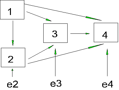
There are customs about displays and names of things in path analysis. Arrows show assumed causal relations. A single-headed arrow points from cause to effect. A double-headed, curved arrow indicates that variables are merely correlated; no causal relations are assumed. The independent (X) variables are called exogenous variables. The dependent (Y) variables are called endogenous variables. A path coefficient indicates the direct effect of a variable assumed to be a cause on another variable assumed to be an effect. Path coefficients are standardized because they are estimated from correlations (a path regression coefficient is unstandardized). Path coefficients are written with two subscripts. The path from 1 to 2 is written p₂₁, the path to 2 from 1. Note that the effect is listed first. A path analysis in which the causal flow is unidirectional (no loops or reciprocal causes) is called recursive.

Points to notice:

1. All possible paths from earlier to later variables are included in this particular graph (1 to 2, 3, & 4; 2 to 3, 4, 3 to 4). There are no backward paths (e.g., 4 to 1).
2. The only exogenous variable is 1 (it has no arrows pointing to it).
3. There are 3 endogenous variables here (2,3,4). Each endogenous variable is explained by 1 or more variables in the model, plus an error term (e2 - e4). An endogenous variable can be a cause of another endogenous variable, but not of an exogenous variable.

The assumptions for the type of path analysis we will be doing are as follows (some of these will be relaxed later):

1. All relations are linear and additive. The causal assumptions (what causes what) are shown in the path diagram.
2. The residuals (error terms) are uncorrelated with the variables in the model and with each other.
3. The causal flow is one-way.
4. The variables are measured on interval scales or better.
5. The variables are measured without error (perfect reliability).

Some or all of these assumptions may not be true. More advanced models are used to cope with some less restrictive sets of assumptions. For now, let's assume that the assumptions are true so that we can develop the concepts.

Because we are working with correlations, we can assume that our variables are in standard score form (z scores). For our example, the equations for the four variables are:

Note that the first variable is not explained by any other variable in the model. In path language, e means stray causes, or causes outside the model. The e does not stand for measurement error, which is assumed to be zero. The second variable (2) is due partly to the first variable and partly to error or unexplained causes. Note the correspondence between the path diagram and the equations. Each z is determined by the paths leading directly to it, and not the indirect paths (e.g., there is no mention of p₂₁ in the determination of z₃).

To calculate the path coefficients, we will use observed correlations:

Which is the formula for r with z scores. If we substitute the path equation for z₂, we get:

which amounts to

The first term on the right is , which is the path coefficient times the variance of z₁. The variance of z₁ is 1, because it is in standard form (this is an entry on the main diagonal of the correlation matrix). The second term on the right is the correlation between z₁ and e₂. But we know that this correlation is zero because that is one of the assumptions of path analysis. So, if we are dealing with z scores, the path coefficient from 2 to 1, p₂₁ is r₁₂.

A path coefficient is equal to the correlation when the dependent variable is a function of a single independent variable, that is, there is only one arrow pointing at it from another variable. So we know our first path coefficient, which leads from 1 to 2. If we look at variable 3, we can see that two paths lead to it (from variables 1 and 2). We can compute paths based on the correlations between variables 1, 2 and 3. Because the error terms are uncorrelated with anything, we will conveniently leave them out of the calculations.

after simplifying terms:

At this point, we know r₁₂ and r₁₃, but we still don't know p₃₁ and p₃₂. We can, however, use r₂₃ to create a second equation that will produce a system of simultaneous equations that we can solve for the path coefficients.

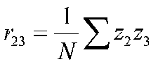
after simplifying terms:

Therefore, we have two equations with two unknowns:

We can solve for p₃₁ by subtracting p₃₂r₁₂ from both sides of the first equation, thus:

Now we can substitute this for p₃₂ in the second equation, thus:

Now we can solve for the sole unknown, p₃₂. With some work, we can show that

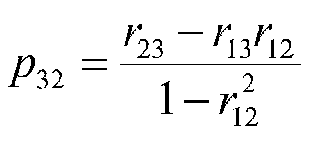
but, incredibly enough, this formula for p₃₂ is the same formula as for a beta weight when we have three variables, and 1 and 2 are the IVs and 3 is the DV. An analogous result holds for the other path coefficient. It turns out, therefore, that the standardized regression weights (betas) solve the problem of the path coefficients nicely.

That is,

Note that this says the correlation between 1 and 3 is equal to the beta for 3 from 1 plus the regression for 3 from 2 times the correlation between 1 and 2. (Look at the path diagram.) The other equation is:

which says that the correlation between 2 and 3 is the regression of 3 on 1 times the correlation between 1 and 2 plus the regression of 3 on 2. (Look at the path diagram.) Note that the path coefficients are beta weights. The first path coefficient was a correlation, but this is also a beta weight when the variables are in standard form because there is only one variable, so r and b are the same.

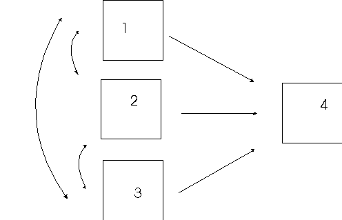
The fourth variable has three paths that come to it (from 1, 2, and 3). We will have to calculate 3 equations to find the unknown path coefficients.

The other two correlations are decomposed as:

The path coefficients can be solved through regression. If we treat variable 4 as our DV and variables 1, 2, and 3 as IVs in a simultaneous regression, we will have the proper beta weights and thus the proper path coefficients.

Recap: path coefficients as beta weights. In our 4 variable problem, we could treat variable 4 as our DV and variables 1, 2, and 3 as our IVs and estimate beta weights for each of them simultaneously. If we did, we would get p₄₁, p₄₂, and p₄₃. If we then toss variable 4 as our DV, and instead take variable 3 as our DV and 1 and 2 as IVs and compute a simultaneous regression, we will estimate p₃₁ and p₃₂. Finally, if we estimate the beta for variable 2 from variable 1 (which is, of course, r₁₂) we have p₂₁. Path coefficients come from a series of multiple regressions rather than from just 1 regression. Or, if you like, regression is the simplest form of path analysis, where we have 1 DV and k IVs, all of which are freely intercorrelated, so that no relations among the IVs are analyzed.

A path diagram implies that correlations are built up of several pieces.

In the correlated cause model (A), part of the correlation between 1 and 3 is due to the direct effect of 1 on 3 (through p₃₁). Part of the correlation will be due to the correlation of 1 with 2, because 2 also affects 3, that is, r₁₂p₃₂. However, we will leave that part unanalyzed because 1 and 2 are exogenous, and therefore the correlation between them is unanalyzed.

In the mediated model (B), only variable 1 is exogenous. We can now decompose all the correlations into direct and indirect effects. In this model, 1 affects 3 directly (p₃₁) but also indirectly through 2 (p₂₁ and p₃₂). The correlation between 1 and 3 can be composed into two parts: direct effects and indirect effects. Some people call the sum of direct and indirect effects the total effect. Now in model B, there will be a correlation between 2 and 3 (r₂₃). This correlation will reflect the direct effect of 2 on 3 (p₃₂). But it will also reflect the influence of variable 1 on both. If a third variable causes the correlation between two variables, their relation is said to be spurious (e.g., the size of the big toe and cognitive ability in children). If the path from 2 to 3 were zero, the entire correlation between 2 and 3 would be spurious because all of it would be due to variable 1. However, in the current example, only part of the correlation between 2 and 3 is spurious. The spurious part is r₂₃-p₃₂ or p₃₁p₂₁.

In model C, the two IVs are independent. In such a case, the path coefficient is equal to the observed correlation.

The observed correlation may be decomposed into 4 pieces:

1. Direct Effect (DE) due to the path from X to Y
2. Indirect Effect (IE) due to paths through intermediate variables
3. Unanalyzed (U) due to correlated exogenous variables
4. Spurious (S) due to third variable causes.

Not all correlations are composed of all four parts, however.

Recall our first figure

We worked out a series of equations, one for each correlation based on this figure:

Because r₁₂ is due to a single path that indicates a direct effect, r₁₂ is composed solely of DE, a direct effect.

What is the point of this decomposition? The point is to better understand the correlations that we observe. How much is due to direct effects, indirect effects and third variables? It may help us to better understand theoretical processes, to gain leverage in the business of change, etc.

Suppose we have 3 variables. The correlations observed among them are:

Suppose our model is:

Because the correlations are decomposed into the 4 kinds of effects, we can build up correlations from path models. For example, for Model

Suppose we have the following model:

We know

p₂₁ = r₁₂ = .60

p₃₁ = b _31.2 = (r₃₁-r₃₂r₁₂)/(1-r₂₁²)=(.50-.40*.60)/(1-.36) = .406

p₃₂ = b _32.1 = (r₃₂-r₃₁r₁₂)/(1-r₂₁²)=(.40-.50*.60)/(1-.36) = .156

Therefore,

p₂₁=.60

p₃₁=.41

p₃₂=.16.

Notice that the path diagram implies a set of equations that allows us to estimate each of the paths. But also notice (new concept) that the path diagram implies a set of equations that would let us estimate a correlation matrix in the absence of data if we knew the path coefficients. In the case of the path diagram we just drew, the correlations are

r₁₂=p₂₁

r₁₃=p₃₁+p₃₂p₂₁

r₁₃=DE + IE

r₂₃ = p₃₂+p₃₁p₂₁

DE + S

Now suppose we didn't have any data, but we did have a theory that said that the following:

p₂₁=.8

p₃₁=.3

p₃₂=.7

Our dependent variable is 3. Our theory says that 3 is strongly predicted by the IVs. Further, most of the effects of variable 1 are explained through the mediating effects of 2.

Our predicted correlations are:

r₁₂=p₂₁ = .80

r₁₃=p₃₁+p₃₂p₂₁ = .3+.7*.8 = .86

r₂₃ = p₃₂+p₃₁p₂₁ = .7+.3*.8 = .94

Notice that we can now collect data, compute a correlation matrix, and compare it to what we predicted based on our theory. This is (to some of us, at least) enormously exiting because we can make quantitative, point predictions and then compare them to actual data. This is analogous to cross-validation. In cross validation we predict values of Y given a previously estimated set of regression coefficients and then compare the predicted values to the actual values. In path analysis, we can generate values of correlations based on a theory and then compare them to actual values. We could actually generate an R-square based on predicted and actual values of r in the off-diagonal matrix. If our predicted and actual values were:

The predicted R is based on our path diagram and associated theory. Suppose we collected data, computed the correlation matrix, and then found the matrix shown under Actual R. As you can see, the correspondence is not very close. To compute r, the correlation between off-diagonal entries, we could find:

Pred Actual

.80 .62

.86 .50

.94 .39

If we compute the correlation between these two columns, we find it to be -.99, which is about opposite to our predictions. However, such an r is not the customary means of evaluating predicted correlations against observed correlations. The problem with such a method of evaluation is that it takes no account of differences in means between the predicted and actual correlations. Instead, the approach typically used in the root-mean-square-residual (RMSR), which is computed by subtracting the predicted from the actual, squaring the result, taking the average over the correlations, and taking the square root. You can think of this as a standard error of prediction or the standard deviation of the residuals. In our data, we have

There are numerous statistical approaches in addition to RMSR to evaluating the fit of path and SEM models. However, they all share the same logic. It is important for you to see the logic of the approach.

1. We assume the values of some parameters based on theory.
2. We estimate the correlation matrix based on the assumed parameters.
3. We compare the observed correlation matrix to that which is based on theory to see how accurate our theory was. That is, we test the fit of the data to the model or theory (using RMSR, c ², or other measures).

It's just...that...simple.

Identification is important for both the estimation of parameters and the testing of model fit.

Parameter estimates. A parameter is said to be identified if a unique, best fitting estimate of the parameter can be obtained based on the sample of data at hand. For example, a path coefficient is identified if a single beta weight is associated with it and the beta weight can be estimated with the given data (sample size is large enough, collinearity is not too severe a problem). A model (path diagram, etc.) is said to be identified if all of the parameters in the model are identified. If a parameter is not identified, it is said to be underidentified, or unidentified, or not identified; same for the model if one or more parameters is not identified. Parameters can be underidentified for many reasons, all of which sort of ruin your day. The most common reason for underidentification (at least in the literature on SEM) is that the set of simultaneous equations implied by the path diagram does not have enough correlations in it to offer a unique solution to the parameter estimates.

For example, suppose my theory says that two variables are reciprocal causes, like this:

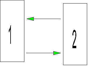
Let's further suppose that it turns out that the predicted correlation between the two variables based on the path model is r₁₂ = p₂₁*p₁₂ (this isn't strictly true, but play along for now). Now let's suppose that the observed correlation between the variables is r₁₂ = .56. We want to estimate p₂₁ and p₁₂. A solution that fits the observed correlation is p₂₁ = .8 and p₁₂ = .7 because .8*.7 = .56. But notice that we could also have p₂₁ = .7 and p₁₂ = .8, because .8*.7 = .56. The problem is that we have two different solutions to the parameter estimates that fit the data perfectly. The data cannot be used to tell which is the better set of parameter estimates. Whenever there is no single, best fitting parameter estimate based on the data, the parameter is unidentified. For our data, p₂₁ and p₁₂ are unidentified because they have more than 1 best fitting solution (parameter estimate).

Model testing. A model is said to be just identified if the set of simultaneous equations implied by the parameters has just enough correlations in it so that each parameter has a solution; if there were any more parameters to estimate, one or more of them would not be identified. If there are some correlations left over after all the parameters have been estimated, the model is said to be over identified. Over identified models have some nice properties for theory testing, which we will get to.

 A just identified model:

An overidentified model:

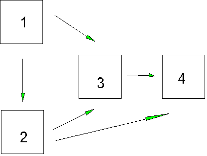
Note that in the overidentified model, one of the paths is missing because it is set to zero (assumed to be zero). If we estimate the parameters of a just-identified model from a correlation matrix, the parameter estimates will always reproduce the correlation matrix exactly (fit will be perfect). If the model is over-identified, the parameter estimates do not have to reproduce the correlation matrix perfectly, and we can compare the observed correlation matrix to the one based on our parameter estimates to examine fit. The closer the two matrices are, the better the model is said to fit the data. Of course, we have to consider how much overidentification there is (the number of parameters assumed by the researcher) in looking at fit because the larger number of parameters assumed, the worse the fit in general.