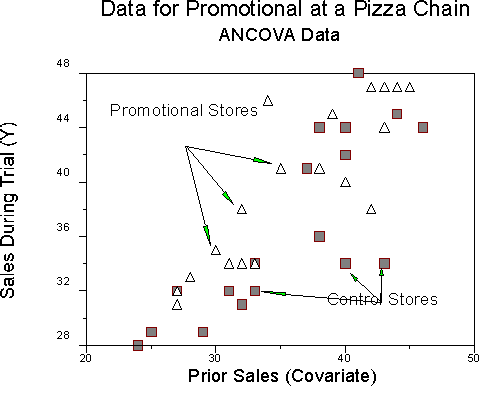
Categorical and Continuous Models 2
What is the difference in philosophy (purpose) between ATI models and ANCOVA models? What is the sequence of tests in ANCOVA? What is the nature of the adjustment in adjusted (least squares) means? Why make the adjustment? What is the difference in interpretation of ANCOVA results when the categorical variable is assigned vs not assigned by the researcher? How do you handle multiple categorical and multiple continuous independent variables in ANCOVA?
Analysis of Covariance
The models in this section (ANCOVA) are identical with those of the last section (ATI, Test Bias) both mathematically and statistically. However, the aim of folks who do this analysis and call it analysis of covariance is quite different than people who do the same analysis and call it aptitude treatment interaction. The primary goal of people who do analysis of covariance is to control statistically within cell variability. If we can reduce within cell variability and keep between cell variability at the same level, we will have a more powerful test. A secondary goal of using ANCOVA is to adjust (between) cell means for differences in the covariate.
For example, suppose we have two methods of teaching research methods to undergraduate psychology majors. In one method, all our examples of statistics come from psychological studies, such as famous studies in social psychology like the conformity studies, bystander intervention studies, etc. In the other method, all our examples come from everyday experience believed interesting to undergraduates, such as the effects of drinking beer on driving a Porsche or the mean number of pepperoni placed on pizzas of equal size by Pizza Hut vs. Dominos. All the students take a common exam, and we look for differences in the means of the two groups to determine whether one method of instruction appears superior to the other. Now we know that some students are more gifted intellectually than are others and that such differences will add to the variability of test scores within groups. If we could remove such variability, we would have a more sensitive test of the difference between teaching methods. ANCOVA will let us do this, that is, to control for differences in cognitive ability to reduce the within cell variability. Note, however, that we DO NOT expect that cognitive ability will interact with teaching method. Another way of saying this is that we expect a common slope for both groups (homogeneity of regression coefficients). ANCOVA doesn't do its job if there is an interaction between the treatment (categorical variable) and the covariate (continuous variable). In such a case, ANCOVA is to be avoided.
If we randomly assign people to each of the instructional methods, we expect that the two groups will be equal (or nearly so) on cognitive ability both before and after the study. The use of ANCOVA will adjust the cell means on the DV for differences in cell means of the covariate. That is, if one group has higher cognitive ability scores than the other, ANCOVA will adjust the research methods test score means (Y) for this difference in cognitive ability (X). If people are not randomly assigned to groups, but instead choose their own method of instruction, and the resulting groups differ in cognitive ability, we have a problem. Now cognitive ability is confounded with treatment. If we use ANCOVA, we can still adjust (control) for differences in cognitive ability across treatments. But if the treatment and the covariate are confounded, we may be reducing the effect size and thus reducing power instead of increasing power. Many people say to avoid ANCOVA if the categorical and continuous variables are correlated. Some people still do it, but there are problems in the interpretation of the results. As in all work with partial and semipartial correlations where we cannot assign people to treatments (cannot assign levels of X), the interpretation of the results is extremely complex. Interpretation of partial correlations should never be done in isolation; such interpretations need to be made under the most thoughtful conditions possible.
My brother and I both used to work for a certain pizza chain. I left to work in a steel factory; he continued to climb the corporate ladder and join the ranks of management. He used to complain about how the company estimated the effects of promotional efforts. They would choose the very best restaurants to try out the promotional (e.g., buy 1 get 1 at half price). They would then estimate the impact of the promotional based on the trial run, and decide to implement it company-wide. Then they would be surprised when the results failed to live up to their estimates. (My brother said that the best managers found ways to make bad ideas work.) What you want to do is to choose two samples of restaurants and randomly assign them to promotional and control. The dependent variable is the store's profit over a time period such as a month. Because of location, management and labor, some stores make a lot more profit on the average month than others. We can control for this to increase the sensitivity of our test to tell whether the promotional makes a difference.
|
Store |
Pre sales (X) |
Trial sales (Y) |
Group (G) |
Store |
Pre sales (X) |
Trial sales (Y) |
Group (G) |
|
1 |
30 |
35 |
1 |
21 |
33 |
32 |
-1 |
|
2 |
28 |
33 |
1 |
22 |
27 |
32 |
-1 |
|
3 |
40 |
40 |
1 |
23 |
38 |
36 |
-1 |
|
4 |
33 |
34 |
1 |
24 |
33 |
34 |
-1 |
|
5 |
45 |
47 |
1 |
25 |
46 |
44 |
-1 |
|
6 |
43 |
44 |
1 |
26 |
40 |
44 |
-1 |
|
7 |
32 |
34 |
1 |
27 |
31 |
32 |
-1 |
|
8 |
38 |
41 |
1 |
28 |
37 |
41 |
-1 |
|
9 |
42 |
47 |
1 |
29 |
44 |
45 |
-1 |
|
10 |
27 |
31 |
1 |
30 |
25 |
29 |
-1 |
|
11 |
31 |
34 |
1 |
31 |
32 |
31 |
-1 |
|
12 |
27 |
31 |
1 |
32 |
29 |
29 |
-1 |
|
13 |
42 |
38 |
1 |
33 |
40 |
34 |
-1 |
|
14 |
35 |
41 |
1 |
34 |
43 |
34 |
-1 |
|
15 |
44 |
47 |
1 |
35 |
41 |
48 |
-1 |
|
16 |
39 |
45 |
1 |
36 |
40 |
42 |
-1 |
|
17 |
32 |
38 |
1 |
37 |
33 |
32 |
-1 |
|
18 |
34 |
46 |
1 |
38 |
38 |
44 |
-1 |
|
19 |
43 |
47 |
1 |
39 |
40 |
44 |
-1 |
|
20 |
27 |
32 |
1 |
40 |
24 |
28 |
-1 |
Note that we have 20 stores in each of two groups (Promo = 1; Control = -1) for a total of 40 stores. Let's take a peek at the data.

We want to know if the promotional has an effect on sales. From SAS PROC MEANS, we find that:
|
|
Dependent Variable |
Covariate |
||
|
Group |
Mean |
SD |
Mean |
SD |
|
Promo |
39.25 |
5.98 |
35.60 |
6.30 |
|
Control |
36.75 |
6.46 |
35.70 |
6.38 |
On the covariate (right columns), we find that the means and SDs are similar for both groups. On the dependent variable (left columns), the mean of sales is about 2.5 points higher for the promotional group than for the control group. Will this be a significant difference? ANOVA "decides" whether a difference is significant by looking at the mean difference in light of the SD and the sample size, N. In this problem, our mean difference is a little less that 1/2 standard deviation.
Well, we can do simple ANOVA without the covariate (that is, Y = a + b1G). If we do, we find that the model has 1 df, with a sum of squares of 62.50, the error term has 38 df, with a sum of squares of 1473.5. Our F is 1.61, which is not significant (p = .21), and R2 is .04.
But we know that lots of the variance in Y is due to location, management and labor effects. We can use prior sales to adjust or control for this. We start ANCOVA by looking for the interaction between the treatment and covariate. If we use PROC REG, we get the following results:
|
Model: |
F=29.78 |
p < .001 |
R2 =.71 |
|
|
|
Variable |
DF |
Par Est |
SE |
T |
P |
|
Intercept |
1 |
8.69 |
3.24 |
2.68 |
.01 |
|
G |
1 |
1.13 |
3.24 |
.35 |
.73 |
|
X |
1 |
.82 |
.09 |
9.18 |
.01* |
|
GX |
1 |
.004 |
.09 |
.05 |
.96 |
As you can see, the model is significant and has a substantial R2. The interaction term is not significant, so we can drop that term and revise our estimates, thus:
|
Model: |
F=45.90 |
p < .001 |
R2 =.71 |
|
|
|
Variable |
DF |
Par Est |
SE |
T |
P |
|
Intercept |
1 |
8.69 |
3.20 |
2.72 |
.01* |
|
G |
1 |
1.29 |
.55 |
2.37 |
.02* |
|
X |
1 |
.82 |
.09 |
9.30 |
.001* |
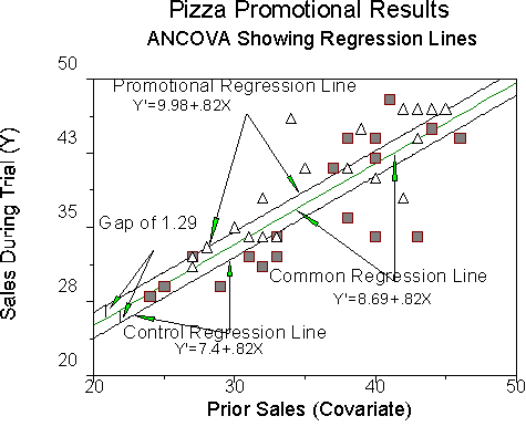
Note that both terms are significant. This means that the promotional has an effect that can be detected after removing the variance due to pre-existing differences in sales among stores within cells. The resulting regression model is one with two parallel lines - identical slopes but different intercepts.
I use PROC GLM rather than PROC REG for this kind of analysis. See the SAS lab manual for a description.
Recap: Our ANCOVA results thus far indicate that there is an effect of the promotional on sales. We can compute the regression lines for the two groups from the results of the REG procedure. Our equation:
Y' = 8.69+1.29G + .82X
We are using the common regression coefficient, bc, which in this case is .82. The b for the group factor modifies the global intercept. For the promotional group, the value of G is 1, so for that group,
apromo = 8.69+1.29 = 9.98, so for this group, the regression line is Y' = 9.98+.82X
For the control group, the value of G is -1, so for that group,
acontrol = 8.69-1.29 = 7.4, so for this group, the regression line is Y' = 7.4+.82X.

Recall that our regression from ANCOVA was Y' = 8.69+1.29G+.82X. Note that the slope for all three regression lines is .82. Note that the intercept of the common line is 8.69, which is the value of a. Note that the gap between each group and the common line is 1.29, which is the value of b for the G term.
Adjusted Means
When analysis of covariance is appropriate, we can adjust the means of the groups on Y for differences in X.
[Technical note: ANCOVA is appropriate when in addition to the ordinary assumptions of regression (approximate normality, homoscedasticity, linearity), we also have
Back to adjusting means. The adjustment is:

where ![]() is the adjusted mean of Group J on the DV,
is the adjusted mean of Group J on the DV, ![]() is the mean of Group J on the DV, b is bc, the common slope,
is the mean of Group J on the DV, b is bc, the common slope, ![]() is the mean of Group J on the covariate, and
is the mean of Group J on the covariate, and ![]() is the grand mean of the covariate, that is, the mean on the covariate over all groups. Note that the formula for adjustment is just like the formula for predicting raw values (not means) in deviation score form, that is,
is the grand mean of the covariate, that is, the mean on the covariate over all groups. Note that the formula for adjustment is just like the formula for predicting raw values (not means) in deviation score form, that is,

In our example, the data are
|
|
X |
Y |
|
Grand Mean |
35.65 |
38 |
|
Promo Mean |
35.6 |
39.25 |
|
Control Mean |
35.7 |
36.75 |
The adjusted means are
For the promotion group:
![]() =39.25-.82(35.6-35.65) = 39.291.
=39.25-.82(35.6-35.65) = 39.291.
For the control group:
![]() = 36.75-.82(35.7-35.65) = 36.709.
= 36.75-.82(35.7-35.65) = 36.709.
Note that the adjusted means are slightly farther apart than the raw means; the promo group's mean is raised slightly and the control mean is lowered slightly. The reason for the adjustment is that the control group started out slightly richer, with better locations and/or more talented people than did the promotional group. ANCOVA can adjust for this difference. If we had done the instructional study in research methods, and found that at the start one group was smarter than the other was, we make an analogous adjustment for cognitive ability. Note that in both cases we randomly assigned people to treatments, so we expect minor adjustments only.
We can test for the differences among the adjusted means, too. There are some really ugly formulas to compute F for the difference. But we won't be using them because it turns out that testing for the difference between adjusted means is tantamount to (my favorite Pedhazur phrase) testing the difference between intercepts of regression lines that share a common slope. Testing for the difference between intercepts turns out to be the same as testing for the difference in b weights for the coded vectors that represent group membership. You remember that the b weight(s) for the G variable adjust the grand intercept up or down for each group, so the b weights amount to differences in intercepts. We can test for the significance of the difference between b weights in the same equation using a method we discussed early on. This method rests on the sampling covariance matrix of the b weights.
Fortunately for us, SAS will do this for us. In our example, I used the code:
|
Code |
Meaning |
|
proc glm; |
Invoke the general linear models procedure |
|
class g; |
Variable G is categorical |
|
model y = g x; |
Regression model for ANCOVA |
|
lsmeans g/ pdiff; |
Give me least squares means (adjusted means) for variable G and test for their difference returning the probability for H0 that the means are equal. |
The result in the SAS output was:
General Linear Models Procedure
Least Squares Means
G Y Pr > |T| H0:
LSMEAN LSMEAN1=LSMEAN2
1 39.2911100 0.0234
-1 36.7088900
Note that the least squares means from SAS agree within rounding error with what I got using the formulas in EXCEL. The p value for the difference is .02, so it is significant by conventional levels as it is less than .05.
More Complicated Models
Thus far, we have only considered the simplest of models, in which there is only one categorical variable with 2 levels and one continuous variable. The generalization to more complicated models is fairly straightforward.

If this F is significant, it means that homogeneity of slopes is not a reasonable assumption, and we stop with the ANCOVA. Just do ANOVA.
5. If this F is NOT significant, we drop the interaction terms, and re-estimate the parameters for the model containing all the main effects plus the interactions among the categorical variables. In our example this model has 10 vectors.

Assuming that the covariates add something to the prediction of Y (that is, the above F is significant), we proceed to look at the interactions and main effects of the model in an analogous fashion with hierarchical regression tests. When we get to cell mean comparisons, we use adjusted (least squares) means.