
Matrix Algebra
What is the identity matrix?
What is a scalar?
What is a matrix inverse?
When (for what kind of matrix) does the transpose of a matrix equal the original matrix?
Carry out matrix multiplication.
Given a matrix and a matrix operation, identify the contents of the resulting matrix (e.g., SSCP, Covariance, Correlation).
Definitions
"A matrix is an n-by-k rectangle of numbers or symbols that stand for numbers" (Pedhazur, 1997, p. 983). The size of the matrix is called its order, and it is denoted by rows and columns. By convention, rows are always mentioned first. So a matrix of order 3 by 2 called A might look like this:
A
=
A matrix called B of order 4 by 4 might look like this:
B
=
By convention, matrices in text are printed in bold face.
Elements (entries) of the matrix are referred to by the name of the matrix in lower case with a given row and column (again, row comes first). For example, a31 = 2, b22=1. In general, aij means the element of A in the ith row and jth column. By convention, elements are printed in italics.
A transpose of a matrix is obtained by exchanging rows and columns, so that the first row becomes the first column, and so on. The transpose of a matrix is denoted with a single quote and called prime. For example A' (A prime) is:
A
=
A' =
Note that A' is not just A "tipped over" on its side (if so, we would see the first column as 1 3 instead of 3 1). It's as if cards or boards with numbers on them for each row were pulled 1 by 1 and placed in order for the transpose. The transpose of B is:
B
=
B' =
(With some matrices, the transpose equals the original matrix.)
If n = k, the number of rows equals the number of columns, and the matrix is square. A square matrix can be symmetric or asymmetric. A symmetric matrix has the property that elements above and below the main diagonal are the same such that element(i,j) = element(j,i), as in our matrix B. (The main or principal diagonal in matrix B is composed of elements all equal to 1.) With a square, symmetric matrix, the transpose of the matrix is the original matrix. A correlation matrix will always be a square, symmetric matrix so the transpose will equal the original.
A column vector is an n-by-1 matrix of numbers. For example:
|
b =
|
.4 |
|
.5 |
|
|
.2 |
|
|
.1 |
(I'm going to use boxes for matrices rather than the standard brackets because of formatting problems.) So, b is a column vector. A row vector is a 1-by-k matrix of numbers. For example,
|
b'= |
.4 |
.5. |
2. |
.1 |
So, b' is a row vector. Note that b' is the transpose of b. By convention, vectors are printed as lower case bold face letters, and row vectors are represented as the transpose of column vectors.
A diagonal matrix is a square, symmetric matrix that has zeros everywhere except on the main diagonal. For example:
|
C =
|
12 |
0 |
0 |
|
0 |
10 |
0 |
|
|
0 |
0 |
5 |
C is a diagonal matrix.
A particularly important diagonal matrix is called the identity matrix, I. This diagonal matrix has 1s on the main diagonal.
|
I =
|
1 |
0 |
0 |
|
0 |
1 |
0 |
|
|
0 |
0 |
1 |
I is an identity matrix. It happens that a correlation matrix in which all variables are orthogonal is an identity matrix.
A scalar is a matrix with a single element. For example
|
d = |
12 |
d
is a scalar.
Matrix Operations
Addition and Subtraction
Matrices can be added and subtracted if and only if they are of the same order (identical in the number of rows and columns). Matrices upon which an operation is permissible are said to conform to the operation.
We are blessed by the fact that matrix addition and subtraction merely means to add or subtract the respective elements of the two matrices.
Addition
|
4 |
+
|
6 |
=
|
10 |
|
1 |
2 |
3 |
||
|
5 |
3 |
8 |
||
|
|
|
|
||
|
x |
y |
z |
Addition
|
1 |
2 |
+
|
3 |
4 |
=
|
4 |
6 |
|
1 |
2 |
5 |
6 |
6 |
8 |
||
|
1 |
2 |
7 |
8 |
8 |
10 |
||
|
|
|
|
|
|
|
||
|
X |
|
Y |
|
Z |
|
Subtraction
|
1 |
2 |
-
|
3 |
4 |
=
|
-2 |
-2 |
|
1 |
2 |
5 |
6 |
-4 |
-4 |
||
|
1 |
2 |
7 |
8 |
-6 |
-6 |
||
|
|
|
|
|
|
|
||
|
X |
|
Y |
|
Z |
|
Multiplication
Unlike matrix addition and subtraction, matrix multiplication is not a straightforward extension of ordinary multiplication. Matrix multiplication involves both multiplying and adding elements. If we multiply a row vector by a column vector, we obtain a scalar.
To get it, we first multiply corresponding elements, and then add them.
|
|
|
|
|
b1 |
=
|
|
|
|
|
a1 |
a2 |
a3 |
b2 |
a1b1 |
+a2b2 |
+a3b3 |
||
|
|
|
|
b3 |
|
|
|
||
|
|
|
|
|
|
|
|
||
|
|
a' |
|
b |
|
c |
|
For a numerical example,
|
|
|
|
|
0 |
=
|
|
=
|
|
|
1 |
2 |
3 |
2 |
0+4+12 |
16 |
|||
|
|
|
|
4 |
|
|
The result of multiplying two such vectors is called a scalar product. Scalar products have many statistical applications. For example, the sum of a variable can be found by placing that variable in a column vector and premultiplying it by row vector made of 1s.
For example
|
|
|
|
|
7 |
|
|
|
|
|
1 |
1 |
1 |
|
8 |
= |
7+8+9 |
= |
24 |
|
|
|
|
|
9 |
|
|
|
|
1'x
= S X
We can find the sum of cross products by such operations:
|
|
|
|
|
1 |
|
|
|
|
|
2 |
4 |
6 |
|
3 |
= |
2+12+30 |
= |
44 |
|
|
|
|
|
5 |
|
|
|
|
x'y
= S XYAnd if we subtract the mean from a column vector, we can find the sum of squares:
|
|
|
|
|
-1 |
|
|
|
|
|
-1 |
0 |
1 |
|
0 |
= |
1+0+1 |
= |
2 |
|
|
|
|
|
1 |
|
|
|
|
x'x
= S x2Unlike ordinary multiplication, matrix multiplication is not symmetric, so that, in general x'y does not equal y'x, that is, pre- and post-multiplication do not usually yield the same result. In general, the first matrix will be of order r1xc1 and the second will be of order r2xc2.
To be conformable to multiplication c1 must be equal to r2. The order of the resulting matrix will be r1xc2. The inside numbers must be equal for multiplication of occur. If they are, the result will be of the order of the outside numbers. Some examples
|
A(1st) |
|
|
B(2nd) |
|
|
AB |
|
|
Rows |
Cols |
|
Rows |
Cols |
|
Rows |
Cols |
|
1 |
5 |
|
5 |
1 |
|
1 |
1 |
|
1 |
10 |
|
10 |
1 |
|
1 |
1 |
|
1 |
6 |
|
5 |
1 |
|
DNC |
|
|
5 |
1 |
|
1 |
5 |
|
5 |
5 |
|
3 |
2 |
|
2 |
3 |
|
3 |
3 |
|
3 |
3 |
|
2 |
3 |
|
DNC |
|
|
2 |
4 |
|
4 |
3 |
|
2 |
3 |
Exactly what happens with matrix multiplication depends upon the order of the matrices (although the pattern of steps is always the same).
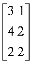
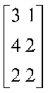
If we multiply a column vector by a row vector, we will get a matrix product of vectors rather than a scalar.
Example
|
1 |
|
|
|
|
|
1 |
-2 |
0 |
|
2 |
|
1 |
-2 |
0 |
= |
2 |
-4 |
0 |
|
3 |
|
|
|
|
|
3 |
-6 |
0 |
|
a |
|
|
b' |
|
= |
C |
|
|
|
3x1 |
|
|
1x3 |
|
|
3x3 |
|
|
Take the first row of a (1), multiply by first column of b (1) set result into to c1,1. Take second row of a (2), multiply by 1st col of b (1), set result to c2,1, etc.
The same pattern is used for larger order matrices, except that for each combination we both multiply and add. For example
|
2 |
1 |
|
|
|
|
|
7 |
8 |
9 |
|
3 |
1 |
|
2 |
3 |
4 |
|
9 |
11 |
13 |
|
4 |
2 |
|
3 |
2 |
1 |
|
14 |
16 |
18 |
|
A |
|
|
B |
|
|
|
C |
|
|
|
3x2 |
|
|
2x3 |
|
|
|
3x3 |
|
|
To get the values of C
|
(2)2+(1)3=7 (1,1) |
(2)3+(1)2=8 (1,2) |
(2)4+(1)1=9 (1,3) |
|
(3)2+(1)3=9 (2,1) |
(3)3+(1)2=11 (2,2) |
(3)4+(1)1=13 (2,3) |
|
(4)2+(2)3=14 (3,1) |
(4)3+(2)2=16 (3,2) |
(4)4+(2)1=18 (3,3) |
Go by the rows of the first matrix and the columns of the second. To get c(1,1) take the first row and first column, multiply the respective elements, and add.
Matrix multiplication is useful to find the matrix of sums of squares and cross products (SSCP matrix).
We can find either the raw score or deviation score sums of squares and cross products. First raw scores:
|
1 |
2 |
0 |
|||||||||||
|
1 |
2 |
2 |
3 |
2 |
2 |
2 |
3 |
2 |
26 |
37 |
14 |
||
|
2 |
3 |
4 |
3 |
4 |
2 |
2 |
4 |
2 |
37 |
58 |
20 |
||
|
0 |
2 |
2 |
2 |
0 |
0 |
3 |
3 |
2 |
14 |
20 |
12 |
||
|
2 |
4 |
0 |
|||||||||||
|
2 |
2 |
0 |
|||||||||||
|
X' |
X |
SSCP |
|||||||||||
|
3x6 |
6x3 |
3x3 |
The contents of the SSCP Matrix
|
|
Sym |
Sym |
|
|
|
Sym |
|
|
|
|
Now deviation scores from the same data:
|
-1 |
-1 |
-1 |
|||||||||||
|
-1 |
0 |
0 |
1 |
0 |
0 |
0 |
0 |
1 |
2 |
1 |
2 |
||
|
-1 |
0 |
1 |
0 |
1 |
-1 |
0 |
1 |
1 |
1 |
4 |
2 |
||
|
-1 |
1 |
1 |
1 |
-1 |
-1 |
1 |
0 |
1 |
2 |
2 |
6 |
||
|
0 |
1 |
-1 |
|||||||||||
|
0 |
-1 |
-1 |
|||||||||||
|
X' |
X |
SSCP |
|||||||||||
|
3x6 |
6x3 |
3x3 |
The contents of the SSCP Matrix
|
|
|
|
|
|
|
|
|
|
|
|
If we multiply or divide a matrix by a scalar, each element of the matrix is multiplied (divided) by that scalar. If we divide each element in the above SSCP matrix by 6 (sample size), we have
|
2/6 |
1/6 |
2/6 |
.33 |
.17 |
.33 |
|
|
1/6 |
4/6 |
2/6 |
= |
.17 |
.66 |
.33 |
|
2/6 |
2/6 |
6/6 |
.33 |
.33 |
1 |
The SSCP matrix divided by N (or N-1) is called the variance-covariance matrix. In it, we have variances on the diagonal and covariances off the main diagonal.
|
|
|
|
|
|
|
|
|
|
|
|
If we further divide through by the standard deviation for each row and each column, we have a correlation matrix:
|
|
|
|
|
|
|
|
|
|
|
|
Correlation matrix for our data:
|
1 |
||
|
.35 |
1 |
|
|
.58 |
.41 |
1 |
Determinants
A determinant is a funky property or value of a matrix. We (well actually, the computer) will be finding the determinants of correlation, variance-covariance, or sums of squares and cross-products (SSCP) matrices. You can think of a determinant as a measure of freedom to vary or lack of predictability in the matrix (I say this to give you some idea of what it is, even if it's not exactly right or precise). Besides a general idea of what it is and its surrounding nomenclature, you need to know (a) that the determinant is used in finding the inverse of a matrix (discussed as the next topic) and (b) what it means when the determinant is zero.
A determinant of matrix A is written
det(A) = |A| or
|
1 |
.5 |
|
.5 |
1 |
|
A |
|
The determinant is denoted by the vertical lines instead of brackets. The determinant is hard to calculate unless the matrix is of order 2x2. In that case, the determinant is just a11(a22)-a21(a12). For our example above, the determinant would be 1(1)-(.5)(.5) = .75.
A large determinant means there is freedom to vary; a determinant of zero means that there is no freedom to vary, there is complete predictability in the matrix. For example, if the correlations among our two measures were 1.0, then the determinant of the correlation matrix would be (1)(1)-(1)(1) = 0. A determinant of zero results when there is a linear dependency in the matrix. That is, if one variable is a linear combination of the other variables in the matrix, the determinant will be zero. For example, suppose I want to use job satisfaction to predict turnover. I have five job satisfaction scales from the JDI (Job Descriptive Index, a famous measure): work, pay, promotions, supervision, and coworkers. Now suppose I want to predict turnover from these five plus overall satisfaction. If I sum the five scales to stand for overall satisfaction, the overall sum will be a linear combination of the five scales (overall=work+pay+promo+super+cowork).
If I put all six scales into a correlation matrix, it will have a determinant of zero. A matrix with a determinant of zero is said to be singular. This is kind of a bad thing, as will be explained soon. Singular matrices pose unpleasant problems for us. A matrix will be singular whenever any two variables in the matrix are perfectly correlated (either r = 1 or r = -1). A matrix will also be singular whenever any variable in the matrix is perfectly predicted by any combination of other variables in the matrix. That is, if we pick any one variable as the dependent variable and we use any combination of other variables in the matrix to compute a linear regression and we find an R2 of 1.0, the matrix is singular. A singular matrix has no inverse.
|
1 |
0 |
0 |
|
|
|
|
|
|
|
0 |
1 |
0 |
|
|A| |
= 1 |
|
|
|
|
0 |
0 |
1 |
|
|
|
|
|
|
|
|
A |
|
|
|
|
|
|
|
|
|
|
|
|
|
|
|
|
|
|
1 |
.5 |
.25 |
|
|
|
|
|
|
|
.5 |
1 |
.25 |
|
|B| |
= .69 |
|
|
|
|
.25 |
.25 |
1 |
|
|
|
|
|
|
|
|
B |
|
|
|
|
|
|
|
|
1 |
1 |
0 |
|
|
|
|
|
|
|
1 |
1 |
0 |
|
|C| |
= 0 |
|
|
|
|
0 |
0 |
1 |
|
|
|
|
|
|
|
|
C |
|
|
|
|
|
|
|
Note that the determinant for A is larger than that for B because there is more freedom to vary in A and, of course, the determinant for C is zero because two of the variables are perfectly correlated.
Matrix Inverse
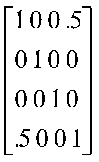
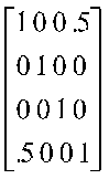
The inverse is the matrix analog of division in real numbers. In real numbers, x-1 is 1/x. And in real numbers, if we multiply x by x-1, we have (x)(1/x)=1. Only a square matrix can have an inverse. The inverse has the property that when we multiply a matrix by its inverse, the results is the identity matrix, I. In other words, AA-1 = A-1A = I. This is special in many ways. First, it is generally not the case that premultiplying and postmultiplying two matrices gives the same result (AX usually does not equal XA). Second, the identity matrix has the property that multiplying it by any conformable matrix results in the same matrix. That is, AI = IA = A. Multiplying a matrix by the identity matrix is analogous to the real number operation of multiplying a number or variable by 1: the resulting output is identical to the numbers input. This is why the matrix inverse is analogous to dividing a number by itself in real numbers. In real numbers, when you divide a number by its reciprocal ('inverse'), the result is 1. When you multiply a matrix by its inverse, the result is I. In both cases (1 and I), multiplying it by something leaves the original thing unchanged.
|
1 |
.5 |
.25 |
|
1 |
0 |
0 |
|
1 |
.5 |
.25 |
|
.5 |
1 |
.25 |
|
0 |
1 |
0 |
|
.5 |
1 |
.25 |
|
.25 |
.25 |
1 |
|
0 |
0 |
1 |
|
.25 |
.25 |
1 |
|
|
B |
|
|
|
I |
|
|
|
BI |
|
|
|
|
|
|
|
|
|
|
|
|
|
|
1 |
.5 |
.25 |
|
1.36 |
-.64 |
-.18 |
|
1 |
0 |
0 |
|
.5 |
1 |
.25 |
|
-.64 |
1.36 |
-.18 |
|
0 |
1 |
0 |
|
.25 |
.25 |
1 |
|
-.18 |
-.18 |
1.36 |
|
0 |
0 |
1 |
|
|
B |
|
|
|
B-1 |
|
|
BB-1 |
||
Verify the multiplication.
BI(1,1) = 1+0+0; BI(2,1) = .5+0+0; BI(3,1) = .25+0+0, etc. BB-1(1,1) = (1)1.36-.5(.46)-.25(.18) = 1; BB-1(2,1) = .5(1.36)-(1).64-.25(.18)=0, etc.
The third, main reason we care about this is that the inverse is used in finding b and b weights from data matrices. If we multiply a correlation matrix by its inverse, we get the identity matrix, I. This lets us multiply both sides of the equation with an inverse to solve a matrix equation (just like dividing both sides of an equation in ordinary algebra).
The inverse allows us to find the b weights.
At any rate, there is no inverse when the matrix is singular (when the determinant is zero). When there is no inverse, we cannot find the b weights. So if we have a singular matrix, we cannot do multiple regression.