Describe the solution for regression weights for raw scores using matrix algebra.

Describe the solution for standardized regression weights from a correlation matrix using matrix algebra.

Describe the sampling distributions of the b and beta weights.

What is the meaning of the covariance or correlation matrix of the b weights? How is it used?

In raw score form the regression equation is:

This says that Y, our dependent variable, is composed of a linear part and error. The linear part is composed of an intercept, a, and k independent variables, X₁...X_k along with their associated raw score regression weights b₁...b_k.

In matrix terms, the same equation can be written:

This says to get Y for each person, multiply each X_i by the appropriate b,_, add them and then add error. The matrices look like this:

With raw scores, we create an augmented design matrix X, which has an extra column of 1s in it for the intercept. For each person, the 1 is used to add the intercept in the first row of the column vector b.

If we solve for the b weights, we find that

To give you an idea why it looks like that, first remember the regression equation:

Let's assume that error will equal zero on average and forget it to sketch a proof:

Now we want to solve for b, so we need to get rid of X. First we will make X into a nice square, symmetric matrix by premultiplying both sides of the equation by X':

And now we have a square, symmetric matrix that with any luck has an inverse, which we will call (X'X)^-1 . Multiply both sides by this inverse, and we have

It turns out that a matrix multiplied by its inverse is the identity matrix (A^-1A=I):

and a matrix multiplied by the identity matrix is itself (AI = IA = A):

which is the desired result.

Suppose our data look like this:

We can represent the regression problem as:

b =(X'X)^-1 X'y

Now to find the inverse of X'X.

If X is a 2 by 2 matrix, then the inverse is a simple function of the elements each divided by the determinant.

Suppose A has the following elements:

Then |A| is ad-bc. The inverse of X is

Or

In our example

And

To find b, we find

Therefore a = -1.38 and b = .54. The regression equation:

Y' = -1.38+.54X.

The raw score computations shown above are what the statistical packages typically use to compute multiple regression.

However, we can also use matrix algebra to solve for regression weights using (a) deviation scores instead of raw scores, and (b) just a correlation matrix. We will, of course, now have to do both.

The deviation score formulation is nice because the matrices in this approach contain entities that are conceptually more intuitive. So let us suppose that we have subtracted the mean of Y from each Y score, and the mean of each X from its column. In that case, we have

which is the same equation as for raw scores except that the subscript d denotes deviation scores. The design matrix X does not contain an initial column of 1s because the intercept for this model will be zero. (Why is the intercept zero?) Because the scores are deviation scores, the matrix X'X will be an SSCP matrix:

And the matrix X'y will be a sums of cross products matrix:

For a two-variable problem, the solution for the b weights looks like this:

This says multiply the matrix of cross products of x and y by the inverse of the SSCP matrix to find the b weights.

The determinant of X'X is found by multiplying the elements of the main diagonal and subtracting the product of the off-diagonal elements. The inverse of X'X is a simple function of the elements of X'X each divided by the determinant.

The b weights will be found by multiplying the above matrix by X'y:

Note that these formulas match those I gave you earlier without matrix algebra.

Recall our 2-variable problem in which we predicted

Chevy mechanics' job performance scores from mechanical aptitude and conscientiousness scores. One of the first things we did was to compute the following matrix:

The table above has sums of squares, cross products, and correlations in it:

To solve for the b weights, we grab the following pieces:

Note that this result agrees with our earlier estimates computed without matrix algebra.

With two standardized variables, our regression equation is

z_y' = b ₁z₁+b ₂z₂

To solve for beta weights, we just find:

where R is the correlation matrix of the predictors (X variables) and r is a column vector of correlations between Y and each X.

Recall our earlier matrix:

The matrix R is:

And the matrix r is:

Therefore our beta weights are:

Note that this result agrees with our earlier estimates of beta weights calculated without matrix algebra.

If the predictors are all orthogonal, then the matrix R is the identity matrix I, and then R^-1 will equal R. In such a case, the b weights will equal the simple correlations (we have noted before that r and b are the same when the independent variables are uncorrelated). The matrix inverse discounts the correlations in r to make them weights that correspond to the unique parts of each predictor, that is, b weights. The inverse operation in a sense makes the predictors orthogonal.

Sampling Covariance of Regression Weights

We can define a population in which a regression equation describes the relations between Y and some predictors, e.g.,

Y'_JP = a + b ₁MC + b ₂C,

Where Y is job performance, a and b are population parameters, MC is mechanical comprehension test scores, and C is conscientiousness test scores. If we take repeated samples from our population and estimate b 1 and b 2, we will have two sampling distributions, one for each slope estimate. Each of the slope distributions will have a variance, known as the sampling variance (this variance is used to construct confidence intervals and significance tests). Because all the variables in this equation are measured on the same people, the measures are dependent. There will be a covariance between the two slope estimates. In other words, the two slope estimates are dependent and may covary (be correlated) across samples. Suppose our population parameters are as follows:

Our population beta weights will be:

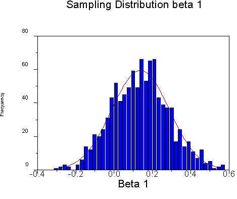
(Note: These b weights are betas both in the sense of being standardized and being population values.) I took 1,000 samples of size 100 from this population. The sampling distribution for beta1 looks like this:

Its mean is .1376, which is close to its expected value of .1388, and its standard deviation is .1496.

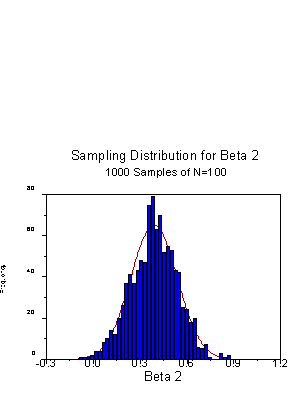
The sampling distribution for beta2 is:

The mean of the distribution is .3893, which is close to the expected value of .3889, and the standard deviation is .1482.

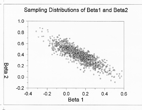
The scatter plot of the pairs of beta weights for the 1000 samples is:

As you can see, there is a negative correlation between the beta weights. When one is relatively large, the other is relatively small. This happens whenever the predictors are correlated. When the predictors are correlated, one predictor tends to get more than its share in a given sample. Correlated predictors are pigs -- they hog the variance in Y.

The variance covariance matrix of the b weights is:

which is the variance of estimate (mean square residual) times the inverse of the SSCP matrix (the inverse of the deviation scores premultiplied by the transpose of the deviation scores). The diagonal elements of this matrix are the sampling variances of the b weights. If we take the square roots of these elements, we have the standard errors of the b weights, which are used in testing them. The off-diagonal elements of C are the covariances of the b weights.

In our example, the sum of squares of error was 9.88. The df was 20-2-1 = 17. Therefore, the variance of estimate is 9.88/17 = .58. The inverse of our SSCP matrix is

Therefore our variance covariance matrix C is

The standard error of b1 is sqrt (c11) = .031.

The standard error of b2 is sqrt(c22) = .046.

The test statistics for b1 and b2 are

t = b1/s1 = .086/.031 = 2.81.

t = b2/s2 = .087/.046 = 1.89.

These t values agree with our earlier calculations made without matrix algebra within rounding error.

To test for the difference between slopes (e.g., is b₁ equal to b₂) includes terms for both the variances of the b weights and also the covariance of the b weights. Specifically,

This test is analogous to a two-sample t-test where we have the standard error of the difference defined as

The difference is that the error variances for the two means are independent, and so the covariance between the two is zero. The b weights are dependent, so we need to include the covariance to be accurate.

In our example

Note: This test is only meaningful when both b weights are of the same kind and measured on the same scale. For example, if one IV were points scored by the home team and the other was points scored by the visiting team for the same type of game this would be okay. But if one were for dollars and one were for days, this would not be okay, because the size of the unit influences the size of the b weight.