Hypothesis Testing
Background
The classical approach to statistical tests, sometimes called Null Hypothesis Significance Testing (NHST), is critical to the process of much of psychological research. It is difficult to get empirical research published, for example, without including some kind of significance test. On the other hand, NHST is increasingly under attack from people that object to the kinds of inferences researchers (and users of research) often make based on the classical approach. Before you can take sides on this issue, you have to understand NHST as a process and mechanism for making decisions. That turns out to be more difficult than understanding most things, and that difficulty is probably why people get into so much trouble when they start making inferences based on the results of statistical tests.
I think NHST is difficult for a couple of main reasons. First, you have to understand the sampling distribution of a statistic under the null hypothesis. “What the heck is that?” you may wonder. We’ll get there shortly. The other thing that’s difficult is that you have to simultaneously consider two things that cannot be true at the same time, and we’re not used to thinking like that. But we can; it’s a bit like learning to ride a bicycle: at first it seems difficult, but once you get it, you always have it and it’s hard to remember when you didn’t have it.
Decision-making under uncertainty
We have to make lots of decisions even though we don’t have all the information. What college or graduate school should I attend? What job should I take? The answer is always something like ‘whatever one is the best for me,’ but that is often difficult to predict. We can, of course, gather information about the choices, and we usually do if the choice is consequential. But we often can’t choose more than one at the same time – we can’t generally accept two competing job offers, for example. That means we can’t compare the options based on our own experience to pick the best for us. However, scientists regularly engage in empirical research so that comparisons are available for our consideration. For example, engineers test automobiles for crash-worthiness, and pharmaceutical companies test drugs for effectiveness.
Origin of Null Hypothesis Statistical Testing
NHST comes from agronomy. Sir Ronald Fisher was stuck in a shed in a field with ledgers full of data about the yield from various crops planted under various conditions. He was hired to make recommendations to farmers about what to plant. You might think for a moment about how you would proceed in his situation (yes, making tea is certainly a good first step). You may have noticed from your own experience that things you plant that ought to grow the same actually don’t. For example, the grass in your lawn might grow well in one spot, but poorly in another. Or you might have planted two of the same kind of tree in two places at the same time and subsequently noticed one thriving and the other languishing. Fisher, being a mathematical genius, worked out a way to take the variability of growth and yield within crops into account when comparing yield between crops and to attach probabilities. The basic idea is to play a ‘what if’ game. What if there is really no difference between crops? What would we expect to see? What would we not expect to see? Right here you might already feel a little uneasy. What do you mean, what would we not expect to see? Well, it’s too soon to worry about that yet. First, we need some statistical jargon to follow what he did.
Statistical Hypotheses
Statistical hypotheses are hypotheses about a population of interest. They are denoted with a capital H, thus H: N(50, 10), meaning that the population is normally distributed with a mean of 50 and a standard deviation of 10. The hypothesis that is actually tested by the process of NHST is called the null hypothesis. By convention, it is written like this:
The other hypothesis, taken to be true if the null is false, is the alternative hypothesis. It is written like this:
Remember, these are statistical hypotheses, meaning that they correspond to characteristics of the population, not necessarily the sample you obtain. We set up the hypotheses so that they are mutually exclusive and exhaustive. In this paragraph, either the population mean is 100, or it is not. Both cannot be true at the same time (mutually exclusive), and between the two, they cover all the possibilities (exhaustive). If we had stated , we would have a problem with the second criterion, because it leaves out means below 100. We could fix this by saying that either the mean is greater than 100, or it is not (that is, the null includes 100 and below, but we’ll ignore this for now).
The Test Process – What if?
Different people describe this differently, but I like to think about the process in four steps.
State the null and alternative hypotheses. For example,
.
I’ll explain more about why we need the alternative as well as the null a bit later.
Specify whatever is necessary to describe the sampling distribution given the null hypothesis. If you don’t know what a sampling distribution is, please go back to the lecture on sampling distributions and read it (or Google it). In addition to the mean, we need to know the standard deviation and the sample size. We may need to specify that the distribution of data in the population is normal as well. So let’s suppose that in the population, the mean is 100, the standard deviation is 10, and we are going to sample N=25 people. If we take endlessly repeated random samples of 25 people from that population, the mean we observe will follow a normal distribution with a mean of 100 and a standard deviation of 10/sqrt(25) = 2. The distribution of such samples is the sampling distribution of the mean.
Find the areas in the sampling distribution that are likely and unlikely to occur if the null hypothesis is true. If the null hypothesis is true, the most likely mean to be observed will be 100, and the vast majority of observed means will fall near 100. The beauty of statistics is that we can state what we mean by likely and carve up the sampling distribution accordingly. Suppose we decide that the likely outcome is the central 95% of the sampling distribution. Because our alternative hypothesis was that the population mean was NOT equal to 100, the other 5%, the unlikely part, we will divide into the very top and bottom 2.5%. We will label the very top and bottom of the distribution as the rejection region. This area (the rejection region) is the place that is possible, but very unlikely to occur if the null hypothesis is true. This is the heart of our ‘what if’ game. What if the null is true? Then the outcome will likely fall close to 100, and we can state precisely how close once we decide on what likely means in this context. Here we decided that likely means 95 percent of the time.
Collect the data and complete the test. Here we would randomly sample 25 people and compute the mean of their scores. If the mean falls into one of the rejection regions, we would declare the result to be statistically significant. If the mean fails to fall in one of the rejection regions, we would declare the result to be non-significant.
To review, NHST is a kind of ‘what if’ game. What if the null hypothesis is true? Well, if it’s true, then we expect to see a result that falls within a given interval or window. If the result falls outside that interval, we reject the null as implausible, and adopt the alternative. In other words, if the result falls in the rejection region, we reject the null in favor of the alternative.
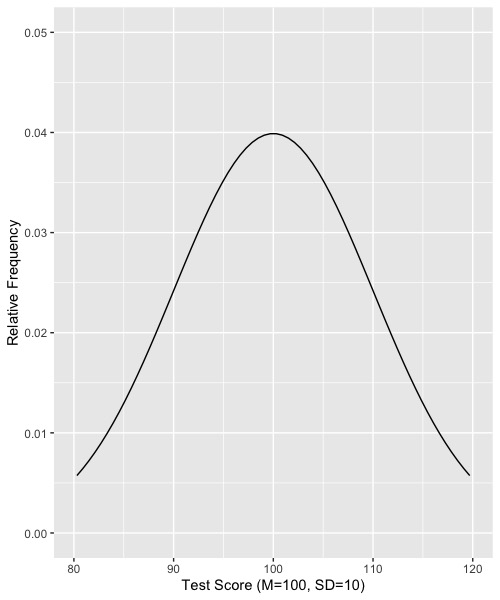
Let’s walk through an example with a graph. Suppose, again that the null is that the population mean is 100, the population standar deviation is 10, and the data are normally distributed. The distribution of raw data in the population would like this:
Now suppose that we draw random samples of size N = 25 from this distribution and compute the mean for each of the samples of N=25. The resulting distribution would look like this:
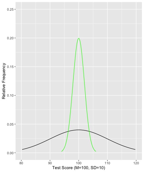
Note that I kept the original (raw data) distribution, which is drawn as a black like. The green line shows the sampling distribution of means given the null hypothesis and samples of N=25.
Now we need to find the rejection regions. Because the sampling distribution of means is normal, we can refer to the normal distribution (z, or unit normal) to find the middle 95% and thus the cutoffs or borders of the rejection regions. The central 95% of the unit normal is found by marking off 1.96 standard deviations above and below the mean. In our example, that would mean 1.96 standard errors, where the standard error is the standard deviation of the sampling distribution. In our case, the value would be 1.96*2 = 3.92. So we would march up and down almost 4 units from 100. One border would be 100+1.96*2 = 103.92, and the other border would be 100-1.96*2 = 96.08. If we draw in our borders and rejection regions, the graph looks like this:
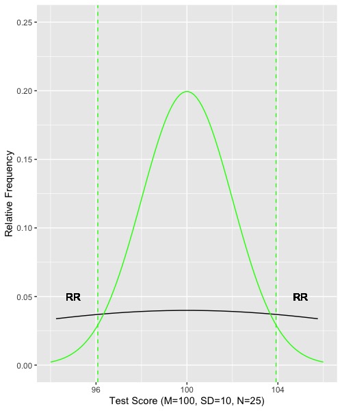
I’ve left the black line for raw data in the graph just to remind you that we are not dealing with the distribution of raw data. Rather we are dealing with the distribution of means. The means are computed on random samples drawn from the raw data. Notice that the rejection regions are a pretty small part of the sampling distribution of means and thus are rather unlikely. We could get a result (value of a mean) in one of the rejection regions just by chance, but it wouldn’t happen very often. In fact, we expect it to happen only 5 times in 100 trials.
Now suppose we collected some data from our actual sample of 25 people, computed the mean for them, and found the value of their mean to be 85. Such a value is in one of the rejection regions, and thus we would conclude that the null hypothesis (population mean = 100) is unlikely to be true. We would declare the result to be statistically significant and reject the null hypothesis. On the other hand, if we collected data and found the observed mean to be 102, the result would not fall into one of the rejection regions. A result of 102 is rather likely if the null hypothesis is true. Thus, in that case, we would declare the result to be non-significant (n.s.), and fail to reject the null hypothesis.
Now you know the process of null hypothesis significance testing as it applies to tests of the mean when the population characteristics are considered known. As you will see, the process is a little more complicated when we have to estimate things rather than considering them known, but the logic is the same; the four basic steps describe the process no matter what.
A Philosophic Difference
There is a difference between making a decision about what to do and making an inference about what is true. Suppose you are trying to decide which of two jobs to take, or which of two cars to buy. You gather what evidence you can, and you make a decision. Your decision is something of a gamble. You choose the option that you think is best, but there is still some uncertainty about your choice. Or suppose you decide what strain of wheat to plant based on an agricultural experiment. You pick the stain that showed a significant improvement in yield over what you had been using. But as you saw in the graph, there is a small chance that the strain you picked is actually no better than last year’s strain. And if it costs more to plant, then you made a poor choice. The point is that when we choose, we act as if we know the population values. We treat a significant difference as if one choice is better than the other. We treat a nonsignificant difference as if there were no difference in the population values. This is the logical thing to do! Suppose you are given the chance to bet on whether a pair of dice will roll a total of 4 or higher vs 3 or lower. If there is even money on the bets, you would take the 4 or higher because it is much more likely. Of course, every now and then the total will be 3 or 2, and if so, you lose the bet. But the smart money bets 4 or higher. So even though there is uncertainty in the future outcome, we choose to act as if we were certain. But if the result is statistically significant, it just means that the obtained result is unlikely given that the null hypotheis is true. And if the result is not significant, it doesn't mean that the null is true, it just means that the null COULD have produced the result. There are different values that could have produced the observed result as well.
In my opinion, then, using statistical significance testing as I’ve described it to you is a good approach to decision making, for example, choosing the appropriate drug for a specific illness, which of two training programs to implement, which of two advertisements is more effective, and so forth. But it’s just the smart way to bet. It doesn’t tell you the truth of the matter. Sometimes the conclusion from NHST is wrong just because of sampling error. Sometimes we are unlucky. Because there is natural variation in how well crops grow, in how quickly we recover from illness, in how well we learn new concepts, and how persuasive we find advertisements, sometimes we will sample unrepresentative people by bad luck and our study conclusion will be mistaken. We need to keep this in mind when we are designing our studies and interpreting our results.
Decisions, Right and Wrong
When we run a statistical test, we will either reject the null hypothesis or not. In the population, the correct conclusion is to reject or not, because in the population, the null hypothesis is either true or false. There are two ways our decision can be right, and two ways that we can be wrong. If the null is true in the population and we fail to reject it, then we made the right call. If the null is false in the population and we reject it, we also made the right call. But if the null is true in the population and we reject, we made a mistake, and if the null is false in the population and we fail to reject, we also made a mistake. I’ll make this less abstract in a couple of ways.
First, the smoke detector. Most houses have a smoke detector that sits quietly in a hall somewhere, patiently waiting for a fire. In case of fire, it is supposed to detect the smoke and sound a loud alarm, which is the cue for people to evacuate. It has that effect on my cats as well, I’ve noticed. Now, either there is a fire, or there is not. And either the smoke detector goes off, or it does not. Let’s look at the possibilities.
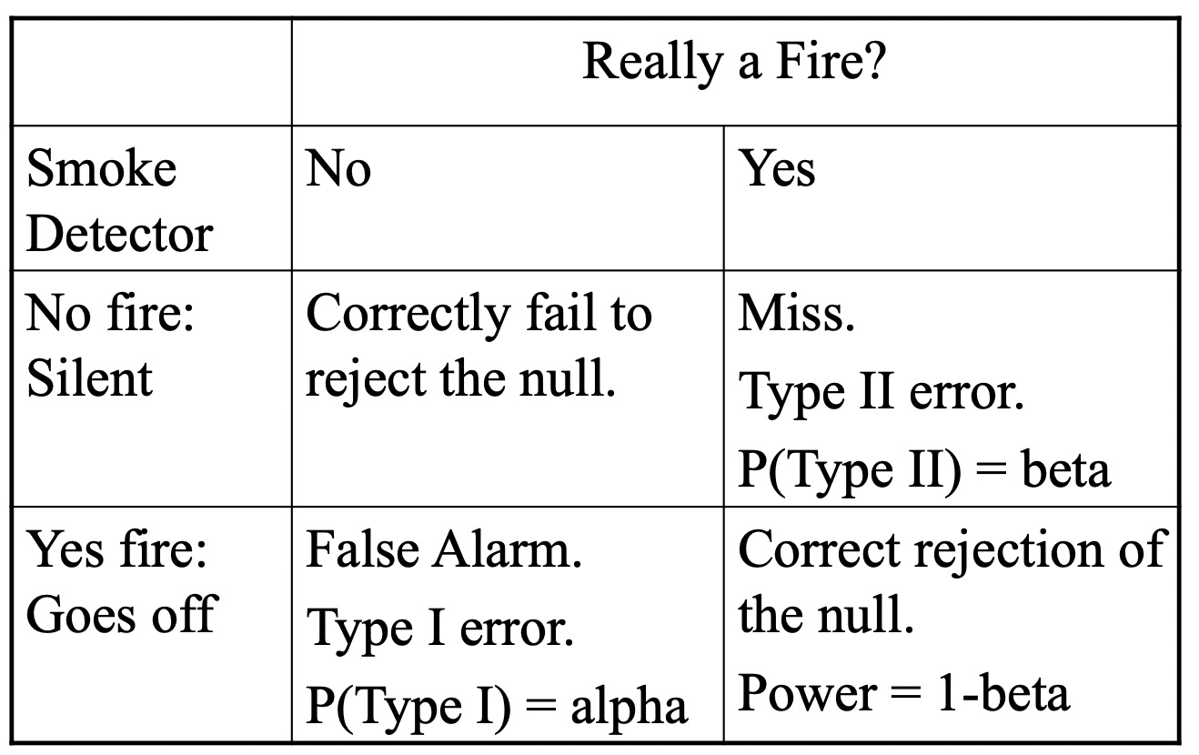
Suppose that there no fire (the usual state of affairs). If the alarm sits quietly, all is well. But if it goes off, that would be called a false alarm. In statistics, that is called a Type I error. We reject the null, but the null is true. The probability that we will make a Type I error is called alpha. You, the researcher, will set the value of alpha by choosing the size of the rejection region. If we put 5% of the area into the rejection region, alpha will be .05 because 5 times in 100 we will reject the null when it is true. Notice that there can only be a Type I error when the null is true, and we started by supposing that there was no fire (the null is true).
Now suppose that the null is false, and that there is a fire. If the alarm remains silent, then it misses the signal. This is a bad thing to happen as you can well imagine, and seemingly worse than the Type I error in this example. The Type I will cause you to grumble or perhaps curse; the Type II may cause your death. The probability of a Type II is called beta. Beta depends on several factors that we will get to shortly. The remaining cell is what happens when there is a fire and the alarm sounds. This corresponds to a correct rejection of the null hypothesis in statistics. The probability of a correct rejection is called power, and can be computed by 1-beta (the opposite of the Type II error). Notice that you can only have power if the null hypothesis is false.
For a second example, let’s consider the case of an antidepressant drug. Patients will be randomly assigned to either the drug or to a placebo (neither the doctor not the patient will know who got what). After a period of time, the patients will be assessed on their degree of depression. Either the drug works better than the placebo in the population, or it does not. For our null hypothesis, we will assume that the drug is not effective, and thus the sampling distribution of mean depression will be the same for both the placebo group and the drug group. The alternative hypothesis will be that the drug is effective. If the truth is that the drug is NOT effective, then the probability of rejecting the null will be the alpha we set before collecting data (typically .05). Chances are good (95%) that we will find a non-significant result and correctly conclude that the drug is not helpful in treating depression. Now let’s suppose that the drug really IS helpful in treating depression. If we run the study and fail to reject the null, we will have made a Type II error, and the probability of doing so is beta. If we run the study and conclude that the drug is effective, well will again have made a correct decision and the probability of doing so is power.
An aside before going further
Nearly all research is done to refute the null hypothesis. The null is a kind of straw man set up just to be knocked down. We are hoping and planning to reject the null when we start a study because we believe that our theoretical position (or hunch, or application) is worth supporting with empirical data. We think our new psychotherapy is more effective than the old one. We think our new drug is effective in treating depression. We think our training program results in superior computer programming. We do the study to prove it. That means we are mostly concerned with beta and power. Oddly enough, in our reports, we often talk about setting alpha, but we rarely talk about setting beta. One reason things are set up like this is that by doing a really bad study, it’s easy to fail to reject the null. If we wanted to show no difference between groups, we just pick a really small sample and measure the outcomes poorly. Works almost every time. Well, works in the sense of providing a non-significant result. But doing a bad study makes it hard to show a real difference, that is, poor studies result in Type II errors. As I said, the point is to reject the null to show that your idea has merit, has support. Therefore, do good studies. One of the reasons for attending graduate school is the sort of apprenticeship in research design so that you learn how it’s done properly. No matter how smart you are, there will be things that go wrong that you didn’t anticipate. People who have done studies have already encountered some of these things that go wrong, and they can show you how to avoid the worst of the pitfalls. One place where people com.monly estimate and report power analyses is in grant applications. More on this in a bit.
Conventional Rules
Set alpha, the probability of a Type I error. Most set this to .05, but sometimes .01. Strictly speaking, the chosen alpha is good for a single statistical test (e.g., whether the experimental group out-performed the control group). More on this when we get to planned comparisons and post-hoc tests.
Choose the rejection region. If the alternative hypothesis is non-directional (e.g.,
), then place the rejection region on the same side as the alternate (one-tailed test).
Call the result significant beyond the alpha level (e.g., p < .05) if the statistic falls in the rejection region. Otherwise, declare the result non-significant (n.s.).
Power
Let’s return to the ‘what if’ game. We want to consider “what if the null hypothesis is false?” In that case, we can either reject the null, which is the correct decision, or we can fail to reject the null, which is a Type II error. The probability of a correct rejection is called ‘power’ in statistics. Power is the probability of correctly rejecting the null hypothesis, that is, a rejection decision when the null is false. Nearly all research is done to show that the null is false, so we want to run studies with good power. If power is poor, we may run the study and be left with non-significant results. Such a condition has been known to cause grown researchers to cry. Consider, you just spent six to 12 months working on a project in order to support your position. You’ve carefully crafted your arguments, developed the study design, collected the data, input to the computer, cleaned the data to remove any mistakes, run the correct statistical analysis, and then… poof… not significant! Aarrrgh!!! Power calculations are typically done before a study to help with the study design so as to avoid the heartbreak of non-significant results.
Again, power calculations can estimate the power associated with the study design. There are several factors that will influence power, including the sample size, the magnitude of effect, the chosen alpha, and the placement of the rejection region(s). For now, I’ll show you power calculations for tests of two means. The actual calculations will change depending on the particular test of interest, but the general principles will not. To begin, we need to set alpha and we need a specific value for the alternative hypothesis, not a general statement about the alternative. So let’s walk through a specific example to give you the general idea.
Example of Computing Power of the Test of the Difference Between Two Means
Suppose . We set alpha = .05. To specify the sampling distribution for the null hypothesis, we also need to know the standard deviation and the sample size (the standard error of the mean is the standard deviation divided by the square root of the sample size). So let us suppose that sigma = 20 and that we will collect data on 100 people. We can now figure the sampling distribution of the mean given the null is true and find the rejection region. The standard deviation of the sampling distribution is 20/sqrt(100) = 2. Because 142 is larger than 138, we will place the entire rejection region above 138. (If we wanted to be agnostic about the alternative, and 142 were of passing interest, we could split the rejection region above and below 138). To isolate the top 5 percent, we move from the bottom of the z distribution toward the top until we reach z = 1.65, which separates the bottom 95 from the top 5. So our border or boundary of the rejection region will be 138+2*1.65 = 141.3. Let’s look at our graph thus far.
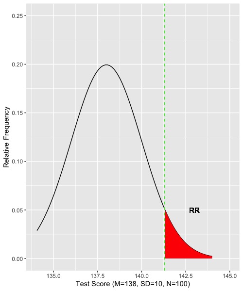
The sampling distribution of the mean given that the null is correct is shown by the black line. The rejection region is colored red. The border is marked by the dashed green line at 141.3. If we collect data, and the resulting mean is greater than 141.3, we would reject the null. Otherwise, we would fail to reject the null. There is half of the story for computing power. Now for the rest of the ‘what if.’
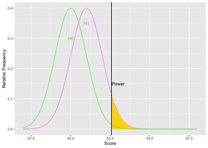
Let’s now suppose that the truth is given by the alternative hypothesis. That is, the mean is really 142 instead of 138. The population standard deviation is still 20 and the sample size is still 100. All is the same except that the value of the mean has changed. First we supposed the mean was 138, now we suppose that it is 142. What would happen here? What would the sampling distribution of means look like under the alternative hypothesis? Let’s look:
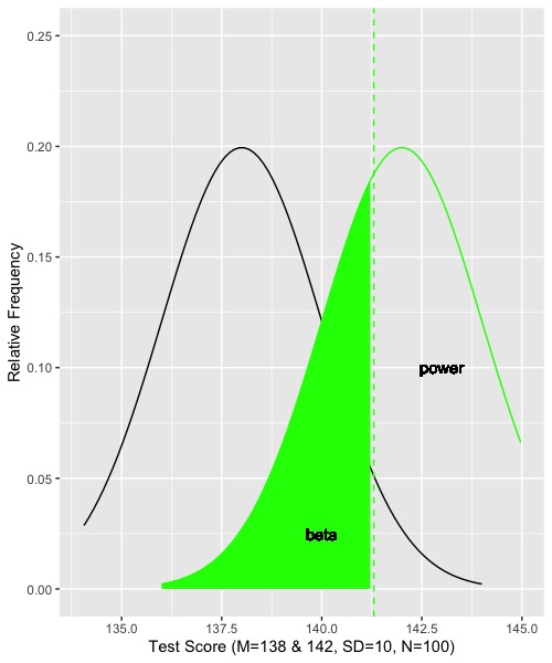
Notice that the dashed vertical green line for the border of the rejection region has not moved. It’s still at 141.3. The sampling distribution for the alternative hypothesis is shown by the solid green line. Every outcome that falls below 141.3 will result in failing to reject the null, even though the null is false. Those are Type II errors, and their probability is beta, which is indicated by the shaded green area. Outcomes that fall above the border (above 141.3) are correct rejections of the null. That probability is power, and it indicated by the portion of the green distribution that is unshaded and labeled ‘power.’ We can find the areas and thus probabilities by referring back to the normal distribution. The z score for the border given the alternative hypothesis is (141.3 – 142)/2 = -.35. If we find the area corresponding to the unit normal and -.35, it turns out to be .36. Therefore, the shaded green portion is 36 percent of the area, and the probability of a Type II error under the alternative is .36. Power is 1 - .36, or .64. That a little better than 50 percent. Not too great.
When designing studies, it is conventional to set alpha at .05 and desired power at .80 (beta = .20). If power is .8, then we have 4 of 5 chances of correctly rejecting the null. You might think that .80 is still too low, especially if you are spending a year of your life on something. Ok, it’s conventional, but not written in stone. We’ll come back to why .80 after I show you the things that affect power: the effect size (choice of population means and variance), the sample size, the rejection region.
Mean Difference
A conventional effect size for mean differences is the standardized mean difference. This effect size depends upon two things: the difference in means, and the size of the standard deviation. The standardized mean difference is denoted
.
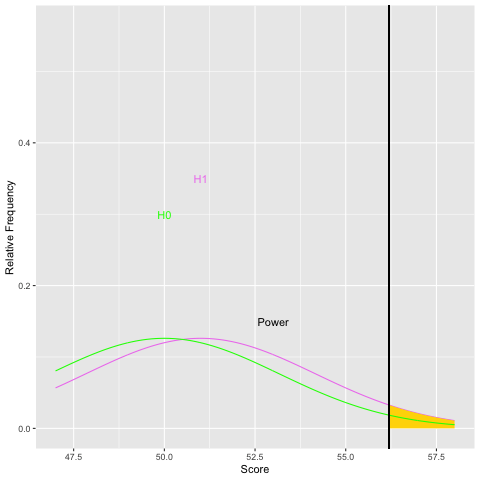
This is quite similar to a z score. First, let’s consider the difference in means between the groups. The larger the difference, the easier it will be to reject the null, and thus the greater the power
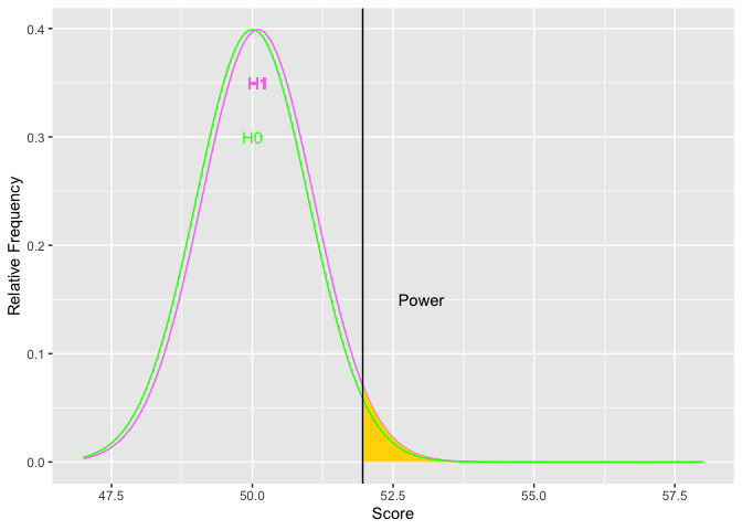
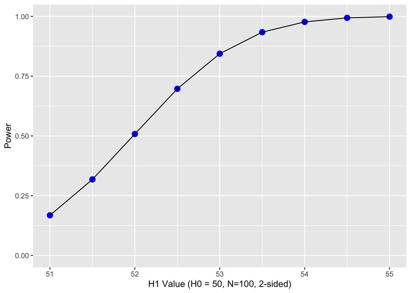
As H1 moves to the right, the difference in means increases (top graph). Simultaneously, the golden shaded area (power) increases. The second graph depicts the relations between the size of the difference (x-axis) and power (y-axis). The limits of power are .05 and 1.00. Based on the normal curve, the limits cannot (quite) be reached because (on the low end) if the alternative hypothesis has the same distribution as the null, then the null is true and there cannot be any power. On the high end, there will always be some possibility of a Type II error because the normal distribution has infinite tails.
The point is that if you have a large difference in means, you are more likely to find a significant result. In graduate school I had a professor who said “go for the whoppers.” What he meant was that we should design studies with very potent independent variables. That way, our studies would come out (would show statistical significance). This remains sound advice today.
Rejection Region
The next item to consider is the rejection region. The things that affect the rejection region are alpha and the placement of the region. Alpha affects the size of the area for the rejection region. The more stringent alpha (going from say .05 to .01), the smaller the area, the fewer the Type I errors (yes!), but also the less power (oh, no!). The border or edge of the rejection region moves away from the mean of the null hypothesis as alpha becomes more stringent. Using a one-tailed test provide more power if the tail is on the correct side. Otherwise, it provides less power. Putting the rejection region on one side moves the border of the rejection region closer to the mean of the null hypothesis. Let’s look at an example.
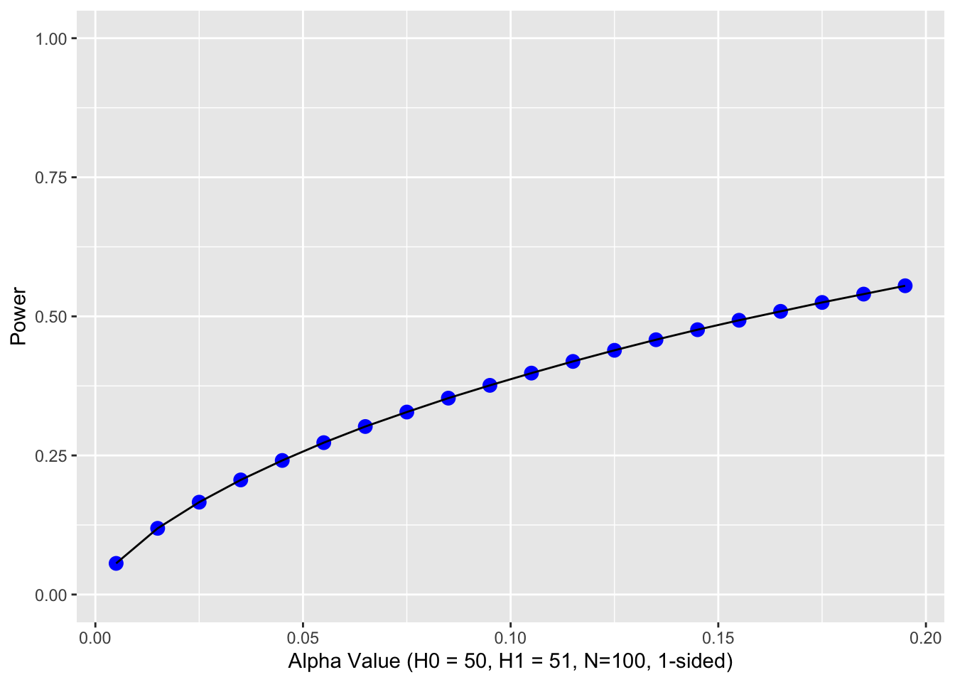
Notice how as alpha increases, the border of the rejection region retreats toward the mean of the null, thus increasing power. The second graph shows an example the relations between alpha and power. You could get power to go even higher, but you would have to increase the probability of a Type I error over 50 percent. Doing so would get you laughed out of stats court.
In theory, you are free to choose any value of alpha that you consider appropriate for your research question. In practice, values other than .05 and .01 are met with skepticism. For values larger than .05, reviewers and readers are apt to think that you decided on alpha after you got your data in order to make the result significant (such a practice is considered unethical; you are supposed to set up the test before you collect the data). However, if you have good reasons for doing unusual things (like setting alpha to .10), you can register your experiment online before you collect data in order to prove that you didn’t decide alpha after the fact. But it’s probably not worth it; there are other things you can do that are a better investment of your energy. Keep reading.
Sample size and Population Standard Deviation
Both the sample size and the population standard deviation influence the standard error of the mean. As a reminder, the standard error of the mean is , which means that the standard deviation of the sampling distribution gets narrow if the standard deviation in the population is narrow and if the sample size is large. You have the greatest control over the sample size – you decide how many participants to include in your study. Most people computing power calculations do so to determine the sample size they need for their study. However, you do have some control over the population standard deviation. The more reliable your measures are, the less error variance they contain, and that results in a smaller the standard deviation in the population. For another example, laboratory animals (e.g., rats) are often bred to be as genetically similar as possible. In doing so, the individual differences among the rats are minimized, and thus the standard deviation in their performance is minimized.
Graphically, as the sample size increases and the population standard deviation decreases, the sampling distribution of the mean becomes narrower. For a given difference in means, as the standard error gets small, the difference becomes more pronounced. Statisticians use the within group variability (here the population standard deviation) as a yardstick to evaluate the size of the difference in means. Let’s examine what increasing the sample size does to power graphically:
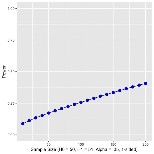
As you can see from both graphs, increasing the sample size increases power. Because sample size is easier to control than some other aspects of study design, it is often the focus of power analyses.
Recalling Two Earlier Points
When I described gaining power by relaxing alpha, I told you that there were better investments for your energy. One of those is recruiting a bigger sample. Another is going for the whopper. When you are starting on a new research program where not much is known, make the manipulation or independent variable as strong as you can. If you are investigating something more nuanced (like dismantling an effective therapy or determining which part of a training program is responsible for the benefit of training), then you will need more people. Or the patience to wait to do the study until after you get tenure.
The second point is why set aspirational power = .80? Why not set it higher, say .95 or .99? Most effects in social science are rather modest (e.g., a standardized mean difference of .5 to .6 is typical). For an effect size of that magnitude, you need a fair number of people to get a significant result. You can increase the power of your statistical test to whatever you like if you recruit enough people. Here is the difficulty, though. The standard error deceases by the square root of the sample size. At first you get a good payoff for adding people. But the payoff diminishes as the sample size increases. It gets too expensive in time, energy and money to keep increasing the sample size. Granting agencies (e.g., NSF, NIMH) supply funds to researchers for projects that the agency finds meritorious. There is only so much money to go around, so they must choose which projects to fund. The agency wants to see that your study has enough people to provide good power, but doesn’t want to pay the extra amount to achieve near certainty. That’s why .80 is the convention. If you are doing a simple study online (e.g., a survey using MTurk) and you have some funds, you can collect data on hundreds of people, and thus crank up the power past .80. But funding agencies don’t like to pay for extra participants.
Summary
NHST is a kind of ‘what if’ game. “What if,” asked Fisher, “the crops really provide equal yields? How different might we expect the observed yields to be?” If the null hypothesis is true, we expect the results of our study to fall within a certain window, interval or boundary. When we do a study, we are hoping that our results will fall outside the window and thus allow us to declare, exclaim, and generally carry on that our results are statistically significant. Given that the null is false, the probability of rejecting the null is called power. We want good power in our studies, so we tend to do the following kinds of things: set alpha as leniently as reasonable (typically .05), use one-tailed tests given a directional alternative hypothesis, work with potent, high-impact independent variables, reduce unnecessary variability in outcome measures by using reliable measures and homogenous populations, and gather large samples. Depending on the design and the statistic of interest, there will be other variables that influence the power of the test. We will discuss those as they arise.