Jargon & Basic Concepts
Discrete vs. Continuous Fuctions
Discrete functions take only specific values (integers;1, 2, 3, etc.). There are no values in between. You have some brothers and sisters (e.g., 0, 1, 2). You don’t have 2.5 brothers (okay, never mind second marriages, adoptions, and all that). Continuous functions take continuous values such that between any two values is always a third. Between 1 and 2 is 1.5. Between 1 and 1.5 is 1.25 and so on. Height and weight are continuous, at least conceptually. In practice, there are limits to the precision of measurement. Mathematically, continuous and discrete functions are worlds apart. People who specialize in one typically have little to say to people who specialize in the other. Discrete functions are typically easier to introduce and to understand as the basis of probability theory. On the other hand, the functions we typically use are continuous. A discrete function we will use: the binomial. A continuous function we will use: the normal.
Sample space
A sample space is the set of possible outcomes of an experiment or process. If we flip a coin once, the sample space is H or T (heads or tails). A sample space for height of adults in the U.S. is all possible height measurements that might be taken (hard to say for sure, might be from about 3 feet to about 8 feet). A sample space is important for statistical work because notions of probability come from comparing what is (our result) and what is possible (the sample space). For example, in a deck of cards, the sample space for dealing a single card has 52 values. The probability of drawing an ace of any sort or an ace of spades is compared to the 52 possibilities (4/52 for aces, and 1/52 for the ace of spades).
Distribution
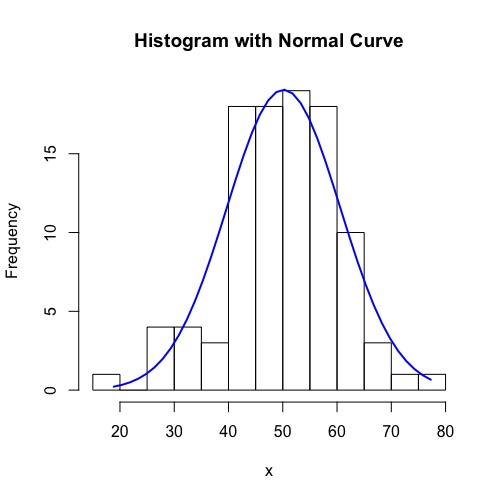
A distribution is an array of scores on a single variable, e.g., measures of height, weight, classroom test scores, MMPI scores, rat bar presses, Beck Depression Inventory scores, Wonderlic scores, etc. It typically refers to a collection of data..
Probability
According to the frequentist view of statistics, probability refers to the relative frequency in a distribution. There are two variants. With an observed frequency distribution, probability means the relative frequency of scores. For example, if there are 14,000 male students and 20,000 female students at USF, then the probability of drawing (meeting, selecting) a male at random is 14,000/(14,000+20,000) = 14/34 = .41. With a theoretical distribution, probability is the expected relative distribution of scores. For example, with a fair coin, the expected relative frequency of heads is ½. Discrete functions are said to have probabilities; continuous functions have probability densities. In continuous math, the point (e.g., a value of exactly 6 feet on the height distribution) has a probability of zero. There is some probability that people fall between 6 feet and 6 feet 1 inch; you have to specify an interval before there is an actual number of people or instances for the continuous distribution. Not so for the discrete distribution, where there will be frequencies for, e.g., 0 sisters, 1 sister, and so forth.
Bernoulli Process
A process or procedure that has a binary outcome. For example, flipping a coin has an outcome of either H or T (only two things can happen). If we looked at the outcome of tossing a single die and coded whether the result was ‘1’ or ‘not 1,’ this would be a Bernoulli process. If two teams play a game and the result for team 1 is win or loss, this would be a Bernoulli process. On the other hand, if we allow ties, then we have 3 outcomes and we no longer have a Bernoulli process; if the coin lands on its side, same deal. The probability of the desired outcome (H or 1 or win) can vary across trials in a Bernoulli process. The probability that a football team will win against a given opponent can change across the football season as players develop in skill and players are benched due to injury or conduct violations.
Random Variable
A variable where known probabilities are associated with sample outcomes. Another way of saying random variable is that the shape of the distribution of the variable is known. For example, if a coin is fair, we know that the probability of heads is .5. If a distribution is normal, we know that about 95 percent of all scores lie between plus and minus 1.96 standard deviations from the mean. A random variable does NOT mean that nothing can be known about the outcome of a sample. It means that the probability of any observation being drawn is known or can be calculated.
Binomial Distribution
An experiment carried out in such a way that independent trials are made from a fixed Bernoulli process results in a binomial distribution. For example, 10 flips of a fair coin result in a binomial distribution of heads. In 1000 tries of 10 flips, there will be so many instances of 0 heads, so many of 1 head, so many of 2 heads all the way to so many of 10 heads. The binomial is a discrete distribution that is used in solving relatively simple problems in probability, such as problems involving coins, dice and cards. The binomial is also related to the normal distribution.
