The Correlation Coefficient
Questions
Why does the maximum value of r equal 1.0?
Give an example in which data properly analyzed by ANOVA cannot be used to infer causality.
Give an example in which data properly analyzed by correlation (r) can be used to infer causality.
What does it mean when a correlation is positive? Negative?
Why do we care about the sampling distribution of the correlation coefficient?
What is the function of the Fisher r to z transformation?
What is the effect of reliability on r?
What is range restriction? Range enhancement? What do they do to r?
Concepts
There are two major different types of data analysis. One type is applied to nominal or categorical independent variables (ANOVA); the other is applied to continuous independent variables. Continuous variables take on many values (theoretically an infinite number). Examples include such variables as height and weight, scores on tests like the SAT, and scores on measures of sentiment such as job satisfaction. In this class, we will deal mostly with continuous variables. The simplest correlation and regression models assume linear relations and continuous independent and dependent variables.
What is the correlation coefficient?
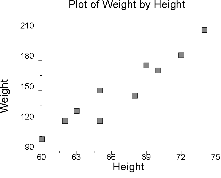
Linear means straight line. Correlation means co-relation, or the degree that two variables "go together". Linear correlation means to go together in a straight line. The correlation coefficient is a number that summarizes the direction and degree (closeness) of linear relations between two variables. The correlation coefficient is also known as the Pearson Product-Moment Correlation Coefficient. The sample value is called r, and the population value is called (rho). The correlation coefficient can take values between -1 through 0 to +1. The sign (+ or -) of the correlation affects its interpretation. When the correlation is positive (r > 0), as the value of one variable increases, so does the other. For example, on average, as height in people increases, so does weight.
|
1 2 3 4 5 6 7 8 9 10 |
60 62 63 65 65 68 69 70 72 74 |
102 120 130 150 120 145 175 170 185 210 |
|
|
|
|
|
Example of a Positive Correlation |
If the correlation is positive, when one variable increases, so does the other.
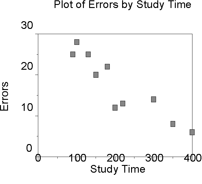
If a correlation is negative, when one variable increases, the other variable descreases. This means there is an inverse or negative relationship between the two variables. For example, as study time increases, the number of errors on an exam decreases.
|
N
1 2 3 4 5 6 7 8 9 10 |
Study Time Min. 90 100 130 150 180 200 220 300 350 400 |
# Errors on test 25 28 20 20 15 12 13 10 8 6 |
|
|
|
|
|
Example of a Negative Correlation |
If the correlation is negative, when one variable increases, the other decreases.
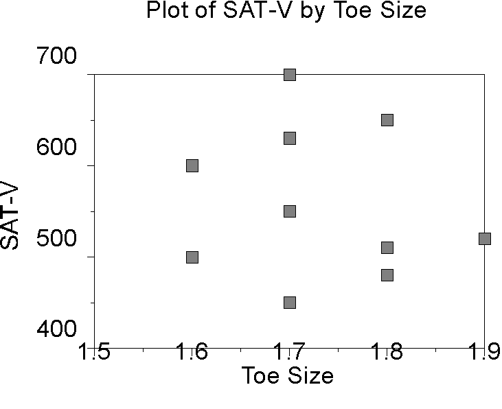
If there is no relationship between the two variables, then as one variable increases, the other variable neither increases nor decreases. In this case, the correlation is zero. For example, if we measure the SAT-V scores of college freshmen and also measure the circumference of their right big toes, there will be a zero correlation.
|
|
Note that as either toe size or SAT increases, the other variable stays the same on average.
The conceptual (definitional) formula of the correlation coefficient is:
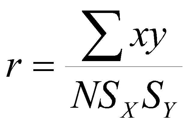 (1.1)
(1.1)
where x and y are deviation scores, that is,
![]() and
and
SX and SY are sample standard deviations, that is,
This says that the correlation is the average of cross-products (also called a covariance) standardized by dividing through by both standard deviations.
Another way of defining the correlation is:
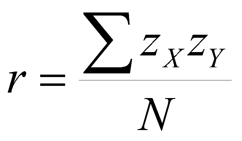 (1.2)
(1.2)
where zx is X in z-score form,
zy is Y in z-score form,
And S and N have their customary meaning. This says that r is the average cross-product of z-scores. Memorize these formulas (1.1 and 1.2). These formulas are equivalent. Recall that

In equation 1.1, x is the deviation score, and SX appears in the denominator. In equation 1.2, SX is divided through and the deviation score appears as zX.
Sometimes you will see these formulas written as:
![]()
and
![]()
These formulas are correct when the standard deviations used in the calculations are the estimated population standard deviations rather than the sample standard deviations, that is, when
![]()
so the main point is to be consistent. Either use N throughout or use N-1 throughout.
Example: Height and Weight Revisited
|
N |
Ht |
Wt |
Zht |
Zwt |
Zh*Zw |
|
1 |
60 |
102 |
-1.4974 |
-1.4344 |
2.1479 |
|
2 |
62 |
120 |
-1.057 |
-0.90424 |
0.95578 |
|
3 |
63 |
130 |
-0.83679 |
-0.6097 |
51019 |
|
4 |
65 |
150 |
-0.39637 |
-0.02062 |
0.00817 |
|
5 |
65 |
120 |
-0.39637 |
-0.90424 |
0.35842 |
|
6 |
68 |
145 |
0.26425 |
-0.16789 |
-0.04435 |
|
7 |
69 |
175 |
0.48446 |
0.715741 |
0.34674 |
|
8 |
70 |
170 |
0.70466 |
0.56846 |
0.40058 |
|
9 |
72 |
185 |
1.14508 |
1.01028 |
1.15685 |
|
10 |
74 |
210 |
1.58548 |
1.74663 |
2.76927 |
|
|
66.8 |
150.7 |
0 |
0 |
.96* |
|
S(N-1) |
4.54117 |
35.9111 |
1 |
1 |
|
|
* The value of .96 comes from dividing the sum of products by 9 rather than 10. I used (N-1) throughout. |
|||||
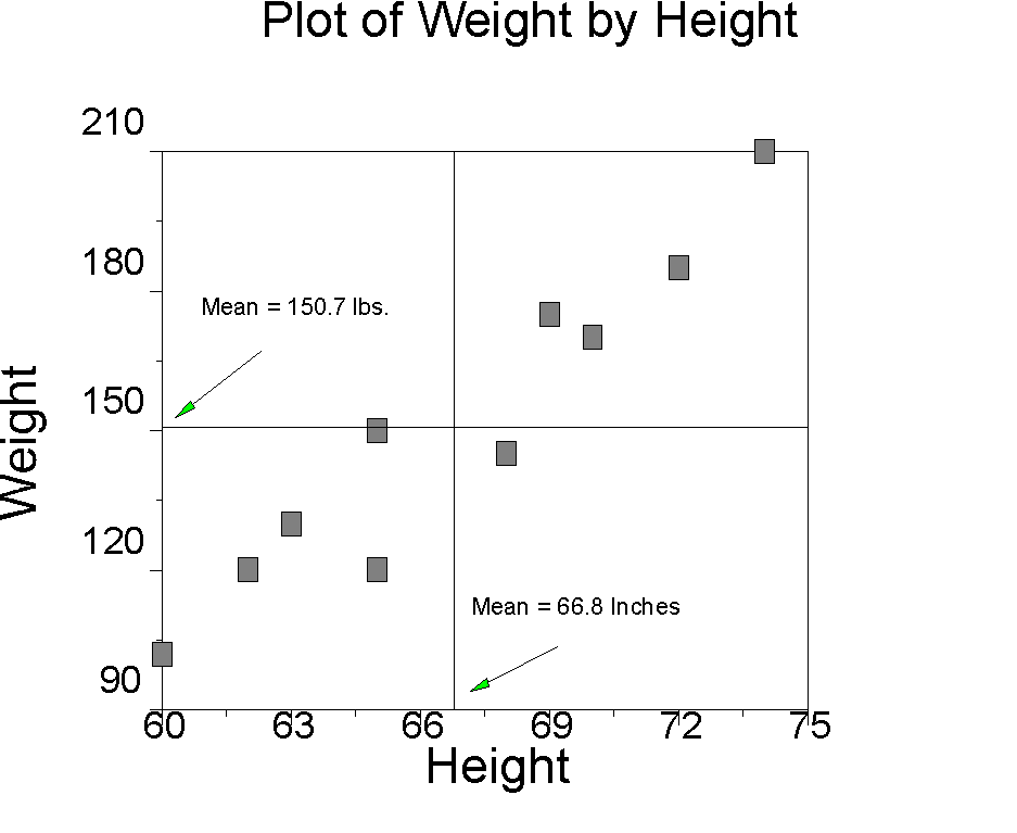
Points to notice: The mean height is 66.8 inches, the SD is 4.54 inches. The first height is 60 inches, which is about 1.5 sample standard deviations below the mean, or a z-score of -1.4974. The first weight is 102 pounds, which is 1.43 standard deviations below the mean weight z = (102-150.7)/35.91 = -1.43. The product of the two z-scores is 2.1479 (-1.4974*-1.4344=2.1479). If we average the products (actually sum and divide by N-1), we get .96, which is the correlation coefficient.
Why does the correlation coefficient have a maximum of 1, and a min of -1? Why is the correlation positive when both increase together?
Let's look at graphs of height and weight. First in raw scores, then in z-scores:
|
|
|
|
Raw Scores |
z-scores |
Points to notice:
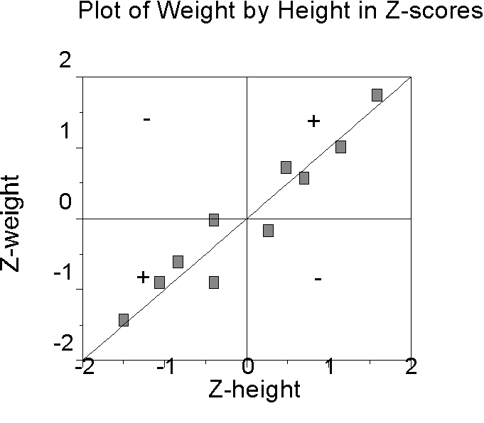
- The pattern or plot of scores is the same in the new and original graphs, but the new mean of height and weight are now zero, and of course the new units are standard deviations.
- Each score is represented by a point, and the points fall into four quadrants defined by the two means. Points in the upper right quadrant are above the mean on both X and Y. Points in the lower right are above the mean on X and below the mean on Y. Points in the upper left are below the mean on X and above the mean on Y. Points in the lower left are below the mean on both X and Y.
- The products of the z-scores will be positive if both zx and zy are positive AND if both zx and zy are negative. Positive cross-products will correspond to points found in the upper right and lower left quadrants. Products will be negative if one or the other, but not both, zx and zy are negative. Negative cross products correspond to points in the upper left and lower right quadrants. Notice that in the z-score graph I have placed a plus sign (+) in the quadrants corresponding to the positive cross-products and a minus sign (-) in the quadrants corresponding to the negative cross-products.
- The correlation coefficient is the average cross- product of z-scores. If most of the points are in the positive quadrants, the correlation will be positive. If most of the points are in the negative quadrants, the correlation coefficient will be negative. If the points are equally distributed in all four of the quadrants, the correlation coefficient will be zero.
- The maximum cross-products occur when x=y, that is, when the points fall on the 45 degree straight line passing through 2 quadrants (either both positive or both negative). This happens because then zx*zy = zx2. For example, if zx is 1, the maximum product obtains when zy is 1 because 1*1 = 1. Any other value less than 1 results in a smaller product, e.g., 1 * .9 = .9. Of course, if zy is greater than 1, then the product is larger than 1, e.g., 1*2 = 2, but this is smaller than if zx had been 2, the same value as zy (2*2 is 4, which is greater than 1*2 = 2). The maximum value of the correlation coefficient (+ or - 1) occurs when the values of x and y fall on a straight line, that is when the co-relation is perfect.
The sampling distribution of r
We don't usually know , the population correlation. We use the statistic r to estimate
and to carry out tests of hypotheses. The most common test is whether
=0, that is whether the correlation is significantly different from zero. For example, we might compute a correlation between a mechanical aptitude test score and a measure of success in a mechanical training program and test to see whether the correlation is different from zero. We can also use r to test whether rho has some value other than zero, such as
=.30. For example, based on past research, we might hypothesize that the correlation between SAT-V and GPA is .60. We can also test whether the correlations are equal across groups (e.g., whether the correlation between SAT-V and GPA is equal for males and females). The tests of hypotheses rest on statements of probability. For example, we might say that the observed r of .70 is very unlikely if
=0. The statements of probability come from sampling distributions. A sampling distribution is what you get if you take repeated samples from a population and compute a statistic each time you take a sample. You might recall that the (long run) average of the sampling distribution of means is the population mean (that is,
, the expected value of the average of the distribution of sample means is the parameter). Another way of saying this is that the sample mean is an unbiased estimator of the population mean. Unbiased estimators have the property that the expected value (mean) of the sampling distribution is the parameter. If the expected value does not equal the parameter, the estimator is biased.
As the sample size increases, the sampling distribution of means becomes normal in shape (this property is known as the Central Limit Theorem). This is really cool because we can use the normal distribution to calculate probabilities and generate tests of hypotheses.
Unfortunately, most of the time the mean of the sampling distribution of r does not equal , nor is the sampling distribution of r ever normal. However, statisticians have developed ways of dealing with this wayward statistic. But first, let's look at the sampling distribution of r. Recall that r is bounded by +1 and -1, that is, it can take no larger or smaller values. When
=0, r is symmetrically distributed about 0, and the mean of the sampling distribution does equal the parameter (yay!). As
increases from zero (becomes more positive), the sampling distribution becomes negatively skewed. As
becomes negative, the sampling distribution becomes positively skewed.
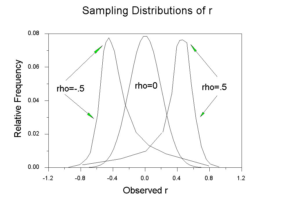
As approaches +1 or -1, the sampling variance decreases, so that when
is either at +1 or -1, all sample values equal the parameter and the sampling variance is zero. The sampling variance of r is approximately
![]()
Note that as | | approaches 1, the sampling variance approaches zero. The shape of the sampling distribution depends on N (trust me on this one). The shape becomes increasingly Normal with large values of N, and becomes increasingly skewed with increasing |
|. As you can see, the sampling variance, and thus the significance test, depend upon (1) the size of the population correlation and (2) the sample size.
The Fisher r to z transformation
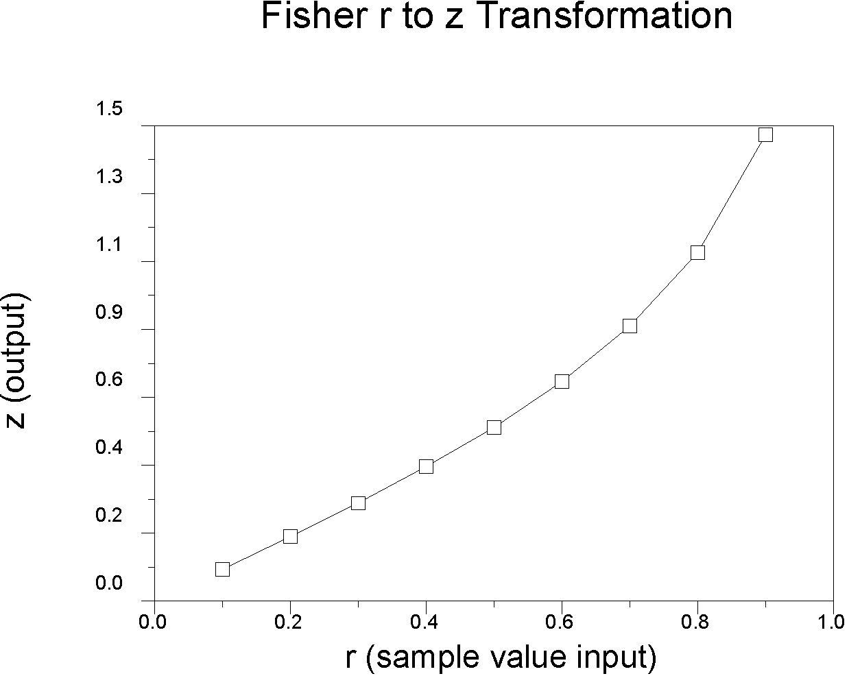
Fisher developed a transformation of r that tends to become normally distributed quickly as N increases; the transformation called the r to z transformation. We use it to conduct tests of hypotheses about the correlation coefficient. Basically what the transformation does is to spread out the short tail of the distribution to make it approximately normal, like this:
|
r .10 .20 .30 .40 .50 .60 .70 .80 .90 |
z .10 .20 .31 .42 .55 .69 .87 1.10 1.47 |
|
Note that r to z doesn't do much until r gets large (the distribution r becomes increasingly skewed as rho increases, so z has to compensate more). The transformation is (e.g., Bishara & Hittner, 2017):
 (1.3)
(1.3)
where loge is the natural logarithm, and r is the sample correlation. The transformation is illustrated above in the table and associated graph.
Testing whether rho =0. SAS (and other statistical package including SPSS and R) use the formula

to compute a value of t and then compare the result to a t distribution with (N-2) df to return a probability value (2-tailed). Look at the p value in your stat package's output to tell if the correlation is significantly different from zero, that is, to test
Testing for a value of other than zero: the one-sample z. Suppose we have done some review work on the correlation between mechanical aptitude test scores and job performance of auto mechanics for Chevy dealers. We know that on average, the correlation is .30. We think our new test is better than this, so we give the test to 200 mechanics and also collect job performance data on them. The resulting correlation is .54. We know that r =0 is not tenable for these data, but we are going to test whether
=.30, that is, H0:
=.30. The formula to do so is:
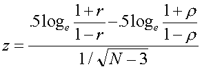 (1.4)
(1.4)
which is distributed approximately as N(0,1) when the null hypothesis is true (that is, we can use the standard normal distribution for probabilities). For our data, we have

 = 4.13
Because 4.13 is greater than 1.96 (1.96 is z or standard normal for alpha = .05, two-tailed), we can reject the hypothesis that =.30 and conclude H1:
not equal to .30. We could have chosen a 1-tailed hypothesis for our alternate H1:
>.30. In that case, we would have used z = 1.645 as our critical value.
Testing the equality of correlations from 2 independent samples. Suppose we want to test whether correlations computed on two different samples (NOT 2 correlations from the same sample) are equal. For example, suppose we compute correlations between SAT-V and freshman GPA separately for samples of male and female students at USF. We find that for males (N=150) r = .63 and for females (N=175) r = .70. We want to know whether these are significantly different, that is, H0: rho 1 = rho 2.
The formula is:
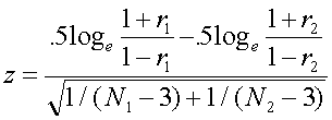 (1.5)
(1.5)
which is distributed approximately as N(0,1) when the null hypothesis is true. For our example

![]() = -1.18, which is not significant because it is contained in the interval -1.96<z< 1.96. We conclude that the correlation between SAT-V and GPA is not different for males and females at USF. Note: this is not a very powerful test (lots of times when there is a real difference, you won't detect it with this test). Also note, we would probably be testing for differences in regression slopes if this were for real. (How to do so will be covered later.) And, yeah, it's phrased as accepting the null hypothesis, which would cause some people to quibble with the diction. Never mind. There may be times, however, when you want to test for differences in independent correlations rather than regressions, and this is how to do it. It is also possible to test whether multiple independent rs are equal. For example, we could test whether the correlation between SAT and GPA is equal across all the state universities in Florida. How to do so is described next.
= -1.18, which is not significant because it is contained in the interval -1.96<z< 1.96. We conclude that the correlation between SAT-V and GPA is not different for males and females at USF. Note: this is not a very powerful test (lots of times when there is a real difference, you won't detect it with this test). Also note, we would probably be testing for differences in regression slopes if this were for real. (How to do so will be covered later.) And, yeah, it's phrased as accepting the null hypothesis, which would cause some people to quibble with the diction. Never mind. There may be times, however, when you want to test for differences in independent correlations rather than regressions, and this is how to do it. It is also possible to test whether multiple independent rs are equal. For example, we could test whether the correlation between SAT and GPA is equal across all the state universities in Florida. How to do so is described next.
More than two independent correlations. Suppose we want to test the hypothesis that three or more correlations from independent samples share the same population value. That is, suppose we have k independent studies and we want to test the hypothesis that rho1=rho2=...=rhok. First we have to estimate the common population value. To do this, we will compute the average across the studies. But first we will use Fisther's r to z transformation. If the studies differ in their sample sizes, then we will also need to compute a weighed average so that the studies with the larger samples get more weight in the average than do the smaller studies. Therefore, we compute:
 ,
,
which is just a weighted average of Fisher transformed correlations. We use (n-3) instead of n because of the z transformation. Now we need to know how far the individual studies are from the average. To get a handle on this, we compute:
![]() .
.
Q is just the sum of squared deviations from the mean where the
squared deviations are weighted by their sample sizes (less 3).
It turns out that when the null hypothesis that all k studies share a
single underlying value of is
true, Q is
distributed as chi-square with (k-1) degrees of freedom. So we can
compute Q and compare the result to a tabled value of chi-square to test
for significance. If Q is large compared to the tabled value of
chi-square, then we can reject the null hypothesis that the study correlations
were drawn from a common population with a single value of
.
For example, suppose we are doing test validation work. We have computed the correlation between bank tellers' performance on a video teller test with customer service ratings furnished by actors in our employ who portray customers with banking problems to the tellers and then evaluate the unsuspecting tellers on their customer service skills. Suppose we have completed studies at three different banks, and we want to test whether the correlation between the test and customer service ratings is the same or different across banks. Suppose we found the following results:
| Study | r | n | z | (n-3)z | zbar | (z-zbar)2 | (n-3)(z-zbar)2 |
| 1 | .2 | 200 | .2 | 39.94 | .41 | .0441 | 8.69 |
| 2 | .5 | 150 | .55 | 80.75 | .41 | .0196 | 2.88 |
| 3 | .6 | 75 | .69 | 49.91 | .41 | .0784 | 5.64 |
| sum | 425 | 170.6 | 17.21 |
The three studies' outcomes or sample rs were .20, .50 and .60. The study sample sizes are shown under the column labeled n. We transform r to z in the next column, which is labeled z. To find the weighted average, we first multiply each z by (n-3), the study sample size less three. When we add the weighted zs, we find the sum is 170.6 The total sample size is 425, which we reduce by nine (reduce n by three for each of the three studies) for a value of 416. Our weighted average, zbar, is 170.6/416 or .41. To find the value of Q, we subtract zbar from each z and square (z-zbar)2. Finally, we weight each squared term by its sample size less three. The weighted, squared entries are shown in the final column of the table. The sum of the entries in the rightmost column of the table is our value of Q, 17.21. We compare this value to chi-square with (k-1) = 2 (in our case) degrees of freedom. The value of chi-square at p = .05 is 5.99, so we can reject the null hypothesis that all studies were drawn from a common population. It appears that the correlation between test scores and customer services is larger at some banks than at others.
Testing for equality of dependent correlations. Suppose you want to test whether two correlations taken from the same sample are equal, that is, you want to test the equality of two elements from the same correlation matrix. There is a literature on this, and there are several available tests. There are two types of test, namely rho12 = rho13 or rho12 = rho34. Note that in the first case, there is one variable in common, and that in the second case, there is no variable in common. An example of the first type would be a test of whether the correlation between cognitive ability scores and performance in a class on U.S. history is equal to the correlation between cognitive ability scores and performance in a class on psychology (same cognitive ability test; two different subject tests). An example of the latter would be whether the correlation between scores on a cognitive ability test and performance on a class test in psychology is equal to the correlation between personality test scores and scores on an interview used to determine a person's suitability for personal counseling as a therapist (whew, what a long sentence). Both types of test are described by Steiger (1980, Psychological Bulletin). For the following hypothesis,
![]() .
.
The Hotelling-William test is:
 ,
,
where
![]()
and
![]() .
.
For example, suppose we have administered a final examination in a statistics class (1). In addition, we have two other measures. One of the measures is the SAT Quantitative score (2), and the other is self-efficacy questionnaire (3) that asks each student how proficient they think they are at various kinds of stats problems. We want to know whether the final exam score is more highly correlated with the SAT-Q or the self-efficacy scale. That is, we want to know whether
![]() .
.
Suppose that we have 101 students in our class. Further suppose that r12 (the correlation between the exam and the SAT) is .4, r13 (exam and self-efficacy) is .6 and r23 is .3.
then
![]()
and
![]()
Therefore
![]()
If we find the critical value for t with 98 degrees of freedom we find the value 1.98. We can therefore reject the null that the correlations are equal in the population. Self efficacy is more highly correlated with our exam score than was the SAT-Q.
It is also possible to test the hypothesis that r 12 = r 34. I once completed a study in which we administered a self-efficacy questionnaire (how good are you at solving problems involving the mean, median or mode?) and an exam (actual problems on the mean, median, or mode) to students in research methods twice, once at the beginning of the semester, and once at the end of the semester. We would expect both self-efficacy and exam performance to increase with instruction. We also expect that students will become increasingly well calibrated over the course of instruction. That is, we expect them to get a better handle on how good they actually are during the semester as they receive feedback on their work. Suppose we have 100 students, and our results look like this:
|
|
1 | 2 | 3 | 4 |
|
1 Self Efficacy Pretest |
1 | |||
|
2 Exam Pretest |
.40 | 1 | ||
|
3 Self Efficacy Posttest |
.30 | .45 | 1 | |
|
4 Exam Posttest |
.10 |
.35 |
.70 | 1 |
If students become better calibrated, then we would expect that the correlation between exam scores and self efficacy scores would be larger at the end of the semester than at the beginning of the semester. We want to test whether the correlations .40 and .70 are significantly different; this will indicate whether calibration improved significantly.
The test that Steiger (1980) recommends for this purpose can be written:

Here z12 and z34 refer to the Fisher transformed values of r, the two correlations. The value in the denominator requires some explanation.
If we define
![]()
then
![]()
and
![]()
In our example, rbar is (.40+.70)/2 = .55. We will substitute the value of .55 for both r12 and r34 in the formula above. Carrying out a bit of arithmetic, we find that
![]()
and
![]() .
.
The transformations of our correlations to z give us .423649 and .867301. Our test, then, is
 .
.
A two-tailed test at alpha = .05 gives us a critical value of 1.96. Therefore, we can reject the null and conclude that the correlations are different. The students became better calibrated over the course of instruction (these are not the data from the article; these are hypothetical data generated to show an example).
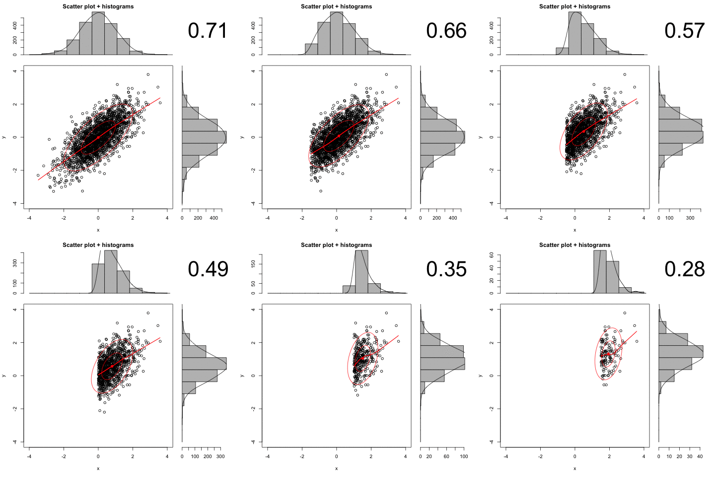
- Range Restriction and Enhancement . Range restriction happens when X, Y, or both are restricted in the values that they can take. For example, suppose we want to know the correlation between a test such as the SAT and freshman GPA. We collect SAT test scores from applicants and compute GPA at the end of the freshman year. If we use the SAT in admissions and reject applicants with low scores, we will have direct range restriction because there will be nobody in the sample with low test scores. There will also be some restriction of range in GPA, because some of the lowest GPA folks will drop out of school during the academic year and so be lost to our sample. Now suppose we do the same study again (that is, correlate the SAT with FGPA) but this time a cognitive ability test other than the SAT will be used for admissions and the SAT will not be used. When we compute our correlation, there will be indirect restriction of range, because the SAT and cog ability test will be correlated, so we will lose a disproportionate number of low ability people from the sample. Some people like to point out that cognitive ability is not important for scholastic success. They say so because in some elite schools like Harvard, there is a minimal correlation between SAT scores and GPA. The result, however is due to restriction of range in SAT -- only higher scoring students get in.
- Enhancement . A. Choose extremes. B. Mix clinical & normal samples but generalize to one or the other.
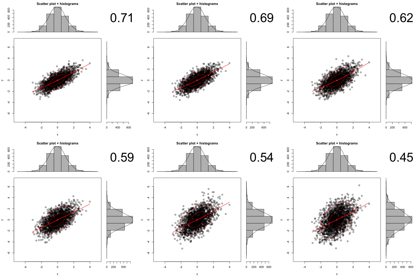
- Reliability . In psychometrics there is an old saying that "reliability sets the ceiling for validity." Reliability describes the amount of error there is in a measure, and validity is often expressed as a correlation coefficient. Reliability coefficients are often expressed as the proportion of true score (the opposite of error) variance in the measure. If all the variance is due to true scores, then the reliability is 1. If all the variance is due to error, the reliability is 0; if half and half, the reliability is .50. (Reliability coefficients are often estimated by alternate forms, test-retest, etc.) A formula that shows how reliability sets the ceiling on validity is:
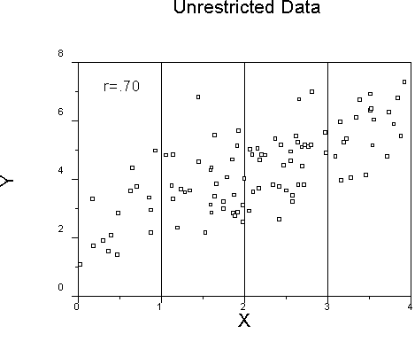
The graph above shows unrestricted data in which both variables are continuous and approximately normally distributed.
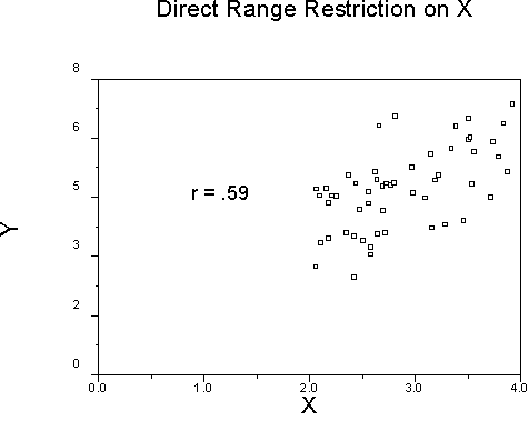
The above graph shows what happens if we delete all cases below the mean on X.
Note how the resulting r is smaller than the original .70.
An animated example:
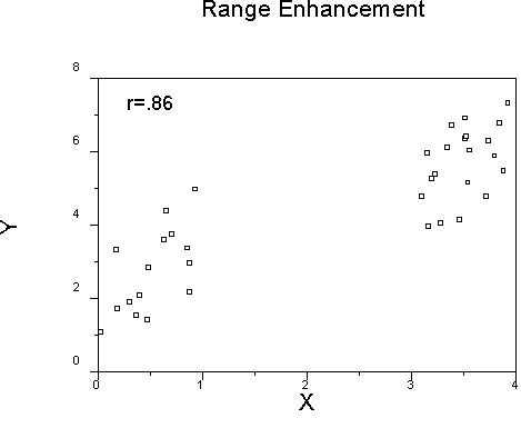
Here we have deleted the observations between 1 and 3. Note how the resulting r is larger than the original .70.

This says that the correlation between observed (measured) variables is equal to the correlation between their true scores, that is, the scores that would be observed with no error times the square root of the product of the two reliabilities, one reliability for each variable. For example, suppose we have a correlation between true scores of .70. The reliability of X is .80 and the reliability of Y is .80. Then the observed correlation will be
r = .70*sqrt(.8*.8) = .7*.8 = .56.
It sometimes happens that we have an observed correlation, estimates of the reliabilities of x and y, and we want to show what the correlation would be if we had measures without error. This is sometimes called a correlation that is disattenuated for reliability. The formula to do this is a simple transformation of the formula above:

For example, if we had an observed correlation of .56, and a reliability of X of .8 and a reliability of Y or .8, then we would have
r = .56/sqrt(.8*.8) = .56/.8 = .70.
An animated illustration of the effect of increasing measurement error:
Distribution Shape
The formula for r is based on the assumption of a bivariate normal distribution. This means that both distributions are normal, and that if you choose any interval of X, the conditional values of Y will still be normal, and if you choose any values of Y, the conditional values of X will be normal. As long as both variables are fairly continuous and more or less normal, r will provide a good summary of the linear relations in the data. However, when one or both variables have a bad shape or have only 2 or 3 values, the range of r becomes restricted. For example, if one variable is binary and the other is continuous, r can virtually never reach a value of 1.0. Its maximum value occurs when about half of the binary values are zero and half are 1, which is also where the maximum variance for the binary measure occurs. The maximum value of r decreases as the proportion of 1s in the binary variable departs from .5. For example, let's look at a few numbers.
|
Person |
X |
Y1 |
Y2 |
Y3 |
|
1 |
1 |
1 |
0 |
0 |
|
2 |
2 |
2 |
0 |
0 |
|
3 |
3 |
3 |
0 |
0 |
|
4 |
4 |
4 |
0 |
0 |
|
5 |
5 |
5 |
0 |
0 |
|
6 |
6 |
6 |
1 |
0 |
|
7 |
7 |
7 |
1 |
0 |
|
8 |
8 |
8 |
1 |
0 |
|
9 |
9 |
9 |
1 |
1 |
|
10 |
10 |
10 |
1 |
1 |
Note that X and Y1 are identical, so the correlation between the two will be 1.0 . Note that Y2 and Y3 are simple transformations of Y1 that make it binary. Y2 transforms Y1 so that values of 5 or less are zero, while values greater than 5 are 1. Y3 transforms Y1 so that values 8 or less are zero. The results:
|
|
X |
Y1 |
Y2 |
Y3 |
|
X |
1 |
|
|
|
|
Y1 |
1.0 |
1 |
|
|
|
Y2 |
.87 |
.87 |
1 |
|
|
Y3 |
.70 |
.70 |
.50 |
1 |
Note that as the binary variable moves from 50 percent, the correlation decreases. Note also that when two things correlate 1.0, they also correlate the same with everything else. Also note that when you correlate two binary variable (Y2 and Y3), the correlation is even lower. There are variants of the correlation coefficient that try to correct for this problem (the biserial and tetrachoric), but there are problems with these (they are only appropriate if the original numbers were dichotomized, and in adition the orignal numbers were normally distributed).
- A measure of association
- As |r| increases, the strength of linear association increases.
- r2 (r-square) is a measure of shared variance, or variance accounted for. If we find that r2xy = .50, we can say that x "accounts for" 50 percent of the variance in y. Or we can say that y accounts for 50 percent of the variance in x, or we can say that they share 50 percent of variance in common.
- Although r2 is the most common interpretation of association (shared variance), r has important interpretations as well. For example, in personnel selection, we can interpret the usefulness of a test using r instead of r2 (the Taylor-Russell Tables are used for this).
2. As a measure of influence
We often talk about experimental (ANOVA) and correlational results as if we can infer cause with one and not with the other. Actually, the statistical analysis has little to do with inferring causality. The important thing for inferring causality is the way in which data were collected, that is, what matters is the design and not the analysis. We can assign people to study time using random numbers with a given mean and standard deviation. For example, before a test we could assign people to receive study time with a mean of 3 hours and a standard deviation of 1 hour, where each person would have a different study time. We could analyze the results with a correlation, and then talk about the influence of study time on test score. On the other hand, we can use ANOVA to test for differences between males and females on test scores, but we cannot say whether any difference in scores is due to sex, gender, specific experience, the absence of chromosomes, etc. Even when we assign people to treatments, we cannot infer causality in the way we would like to. Assignment tends to eliminate alternative explanations of results. There are almost always alternative explanations left even after the assignment. For example, demand characteristics of an experiment may explain the results better than the manipulated variable (that is, the study's participants acted the way they did not because of the manipulated variable, but because they knew they were in a study and it mattered). Remember the Hawthorne studies.
It is useful to think about observed, measured variables as being composites made up of several things, only one of which we typically want to know. For example, suppose we are interested in the association between student satisfaction with school and cognitive ability (loosely, how happy and how smart). Suppose we measure each student's satisfaction with a survey full of items like (my teachers are...enthusiastic, stupid, putrid, helpful; the school facilities are...well lighted, crumbling, smelly, inspiring; overall, my school is ... great, boring, fun, interesting, a waste of time). Responses are summed from strongly disagree to strongly agree; reverse coded, etc. For cognitive ability, we measure student grade point average. Now let's consider what the correlation between the two might mean.
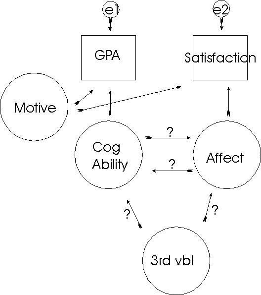
Our correlation will be based on two observed measures, one for satisfaction and one for GPA. Observed measures are represented by square boxes. The observed measures usually don't cause anything, but rather reflect other causes. For example, part of GPA is
due to cognitive ability. Part of our satisfaction measure is due to affective reactions to school (what we want to measure). Both observed measures are subject to errors of measurement (e1 and e2). Both are subject to stray causes (e.g., motives). Now the correlation between the two observed measures could be due to a simple correlation between the things of interest, one causing the other (a to b or b to a), a third variable, or shared errors. This is the difficulty we face when trying to interpret r as a measure of influence.
References
Bishara, A. J.., & Hittner, J. B. (2017). Confidence intervals for correlation coefficients when data are not normal. Behavior Research Methods, 49, 294-309.
Steiger, J. H. (1980). Tests for comparing elements of a correlation matrix. Psychological Bulletin, 87, 245-251.
