What is Importance?

People will ask you about the relative importance of different variables in regression models. You should know that there are many different statistical indices of importance, and that they need not - and usually do not - agree with one another. Becoming an informed consumer of importance measures requires that you to understand to some degree why they disagree. You want to make an informed choice about what you want to compute and to present to others.

There are two broad classes or groups of statistics used to infer importance that correspond to slopes and shared variances. Exemplars of each class are the Pearson’s correlation coefficient, i.e., r_xy, and its square, r². The correlation coefficient is the slope relating Y to X if both variables are measured as z scores (each having mean zero and standard deviation one). The squared correlation coefficient indicates the proportion of variance in Y that is shared with (or accounted for) by X. For linear prediction problems in which importance is most associated with changes in the dependent variable, the slopes are more helpful as importance indicators because they directly translate change in X to change in Y.

For example, suppose we have computed a regression where test scores are regressed on study hours for a given subject matter in a college course. If importance is interpreted in terms of change or difference in test scores, then slopes are helpful because if we increase study hours by 2 hours, mean test scores are expected to change by 2b, where b is the slope. (Of course, we must be mindful about making causal inferences based on correlational designs.)

If importance is interpreted in a more abstract way, then variance is typically preferred. We might want to compare how much variance in test scores is accounted for by study hours, or how the variance in test scores shared with study hours compares with variance in test scores shared with a measure of cognitive ability. Despite the apparent advantage in meaningfulness of the slope, the shared variance is assumed by most authors as the statistical class of interest, so that’s what I will emphasize here. For an overview of importance measures in regression, a readable account is provided by Johnson and LeBreton (2004). There are several more indices than what I present; those presented here are the best of the lot in my opinion.

Description of the Problem

In simple regression, we have one IV that accounts for a proportion of variance in Y. The influence of this variable (how important it is in predicting or explaining Y) is described by r or by r². If r² is 1.0, we know that the DV can be predicted perfectly from the IV; all of the variance in the DV is accounted for. If the r² is 0, we know that there is no linear association; the IV is not important in predicting or explaining Y. With 2 or more IVs, we also get a total R². This R² tells us how much variance in Y is accounted for by the set of IVs, that is, the importance of the linear combination of IVs (a+b₁X₁+b₂X₂+...+b_kX_k). Often we would like to know the importance of each of the IVs in predicting or explaining Y. In our Chevy mechanics example, we know that mechanical aptitude and conscientiousness together predict about 2/3 of the variance in job performance ratings. But how important are mechanical aptitude and conscientiousness in relation to each other? If the independent variables are uncorrelated, the answer is unambiguous. If the independent variables are correlated, however, there are many ways to estimate the importance, so the answer becomes rather murky.

I am going to emphasize four indices of importance for multiple regression:

(a) the squared zero-order correlation,

(b) the standardized slope (often called beta), and the associated shared variance unique to the independent variable (last-in increment),

(c) the standardized slope multiplied by the correlation (beta*r), and

(d) the average increment (statistic used for general dominance).

Background

But first, I am going to introduce Venn diagrams to help explain describe what happens. You should know that Venn diagrams are not an accurate representation of how regression actually works. Venn diagrams can mislead you in your reasoning. However, most people find them much easier to grasp than the related equations, so here goes. We are going to predict Y from 2 independent variables, X1 and X2. Let's suppose that both X1 and X2 are correlated with Y, but X1 and X2 are not correlated with each other. Our diagram might look like Figure 5.1:

Figure 5.1

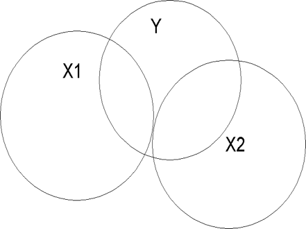
In Figure 5.1, we have three circles, one for each variable. Each circle represents the variance of the variable. The size of the (squared) correlation between two variables is indicated by the overlap in circles. Recall that the squared correlation is the proportion of shared variance between two variables. In Figure 5.1, X1 and X2 are not correlated. This is indicated by the lack of overlap in the two variables. We can compute the correlation between each X variable and Y. These correlations and their squares will indicate the relative importance of the independent variables. Figure 5.1 might correspond to a correlation matrix like the one shown in Table 5.1:

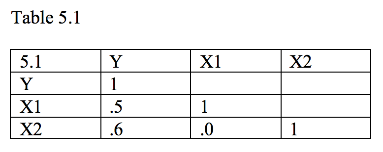
Because X1 and X2 are uncorrelated, we can calculate the shared variance between the two X variables and Y by summing the squared correlations. In our example, the shared variance would be .50²+.60² = .25+.36 = .61. This turns out to be 61 percent shared variance, and if we calculated a regression equation, we would find that R² was .61. If X1 and X2 are uncorrelated, then they don't share any variance with each other. If each independent variable shares variance with Y, then whatever variance is shared with Y is must be unique to that X because the X variables don't overlap.

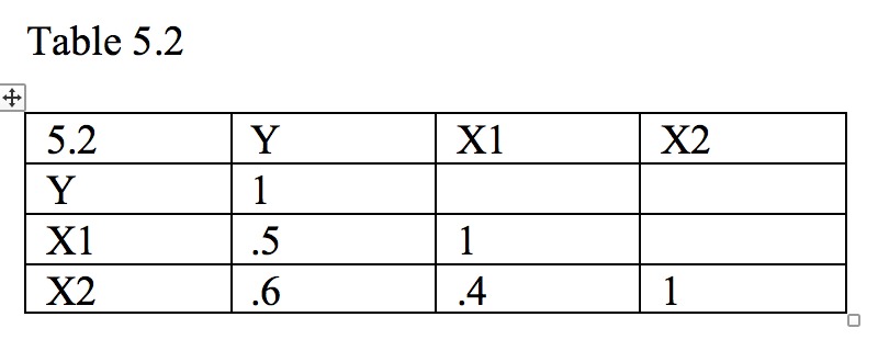
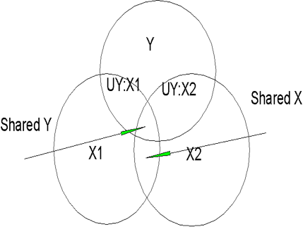
On the other hand, it is usually the case that the X variables are correlated and do share some variance, as shown in Figure 5.2, where X1 and X2 overlap somewhat, as shown in Table 5.2. Note that X1 and X2 overlap both with each other and with Y. There is a section where X1 and X2 overlap with each other but not with Y (labeled 'shared X' in Figure 5.2). There are sections where each overlaps with Y but not with the other X (labeled 'UY:X1' and 'UY:X2'). The portion on the left is the part of Y that is accounted for uniquely by X1 (UY:X1). The similar portion on the right is the part of Y accounted for uniquely by X2 (UY:X2). The last overlapping part shows that part of Y that is accounted for by both of the Y variables ('shared Y').

Figure 5.2

In multiple regression, we are typically interested in predicting or explaining all the variance in Y. To do this, we need independent variables that are correlated with Y, but not with X. It's hard to find such variables, however. It is more typical to find new X variables that are correlated with old X variables and shared Y instead of unique Y. The desired vs. typical state of affairs in multiple regression can be illustrated with another Venn diagram:

Desired State (Fig 5.3)

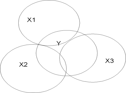
Typical State (Fig 5.4)

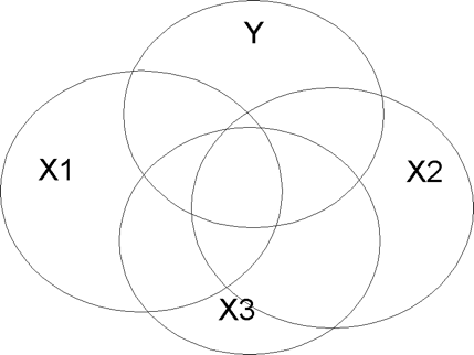
Notice that in Figure 5.3, the desired state of affairs, each X variable is minimally correlated with the other X variables, but is substantially correlated with Y. In such a case, R² will be large, and the influence of each X will be unambiguous. The typical state of affairs is shown in Figure 5.4. Note how variable X3 is substantially correlated with Y, but also with X1 and X2. This means that X3 contributes nothing new or unique to the prediction of Y. It also muddies the interpretation of the importance of the X variables as it is difficult to assign shared variance in Y to any X.

Just as in Figure 5.1, we could compute the correlations between each X and Y for Figure 5.2. For X1, the correlation would include the areas UY:X1 and shared Y. For X2, the correlation would contain UY:X2 and shared Y. Note that shared Y would be counted twice, once for each X variable. If we just add the squared correlations, we would again get .61. We could also compute a regression equation and then compute R² based on that equation. If we did, we would find that R² corresponds to UY:X1 plus UY:X2 plus shared Y. Note that R² due to regression of Y on both X variables at once will give us the proper variance accounted for, with shared Y only being counted once. In Table 5.2, X1 correlates .5 with Y, X2 correlates .6 with Y, and X1 correlates .4 with X2. In this case, the R² for the regression including both independent variables will be .44 instead of .61. To find the unique contribution of each independent variable in Table 5.2, we take the total R² and subtract the R² for each of the constituent variables. Thus, for X1, we have .44 (total R²) less .36 (R² for X2 considered alone) = .08, the unique contribution of X1 above and beyond X2 (UY:X1 in Figure 5.2). For X2 (UY:X2), we have .44 - .25 = .19. Now if we add the unique contributions, .08 + .19 = .27, which is less than .44. The difference is that part of Y that is predicted jointly by X1 and X2. Thus, .44-.27 = .17, which is the shared portion of Y that cannot be attributed unambiguously to either X1 or X2.

An honest answer to a question about variable importance in such a situation might be something along the lines of ‘both variables contribution something unique to the prediction, but a large part of the prediction is shared by both, so I cannot tell you which is responsible for that part of it. That is the nature of correlated predictors.’ But many find such a response to be unsatisfying. Suppose, therefore, that we want to assign or divide up the common part of R² to the appropriate X variables in accordance with their importance. We can do this a couple of ways.

One way is to multiply the standardized regression weights (betas) by the zero-order (raw, unadjusted) correlations (β_i*r_i). In our first example (5.1), the independent variables were uncorrelated, so that the correlation coefficients are equal to the beta weights. Therefore, multiplying beta by r is equal to squaring the correlation coefficient. In our example, we have .5*.5 and .6*.6 or .25 and .36, which sum to .61. In our second example (5.2), the independent variables were correlated .4. The resulting standardized regression weights (betas) are .3095 and .4762. When multiplied by their respective correlations, we get .3095*.5= .15 and .4762*.6 = .29, which sum to .44, the total R².

A second method is to consider all possible increments to R-square when the variable is considered last. In this case, the increments are very simple to calculate. We have the increments when no other variables are in the model, which amount to .25 and .36 in the current example for X1 and X2, respectively. The increments for each variable after including the other first were calculated previously (these are UY:X1 and UY:X2). In our example 5.2, the unique contribution for X1 was .08 and for X2 it was .19. Thus the average increment for X1 is (.25+.08)/2 = .165, and the average increment for X2 is (.36+.19)/2 = .275. In this particular case, the two methods agree substantially, but this is not generally the case. The average of all possible increments is used dominance analysis (Azen & Budescu, 2003).

One way to assess the relative importance of the variables is to compute ratios. The indices, their values for X1 and X2 in Table 5.2 (Figure 5.2), and their ratios are shown in Table 5.3. As you can see, the numerical indices of importance differ, as do their ratios. One could argue that any of them are correct from a mathematical perspective.

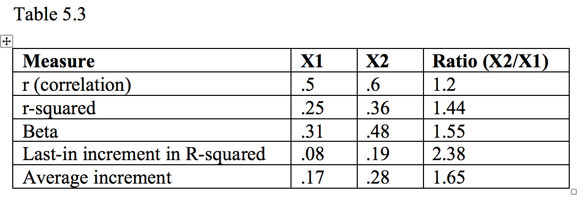
Although there was good agreement in the relative ordering of X1 and X2 in this example, such need not be the case. Having illustrated the four approaches with an example, I’ll now turn to describing the pros and cons of each in a bit more detail.

The squared correlation. Most researchers will present a correlation matrix as a preliminary to computing a regression analysis. Table 5.1 is a very simple example. In the first column of Table 5.1, we see the correlations between each independent variable and the dependent variable. One index of the importance of each variable is simply the square of the observed correlations of each independent variable with the dependent variable. As we saw previously, this worked well for the case in which the independent variables were uncorrelated, but not so well when they were correlated. The squared correlations do indicate the amount of variance that would be attributed to each of the variables if we were to select only one of them. Therefore, such an index would be quite informative should the decision require using only one measure. However, it is hard to imagine a real application with such a restriction. The drawback to using squared zero order correlations as importance indices is illustrated in Figure 5.4, where X3 has no contribution to R-square once X1 and X2 are included in the model.

Beta and incremental R-squared. Raw regression weights (b-weights) are used for making actual (raw score) predictions of the dependent variable given actual values (raw scores) for the independent variables. However, the size of the regression weights will depend upon the scaling of the independent variables. Thus a scale with a large variance (e.g., SAT scores on a scale from 200 to 800) will typically show a smaller b-weight than a scale with a small variance (e.g., high school grade point average on a scale of 1.0 to 4.0). To adjust for scaling differences, we often standardize each variable by subtracting the variable’s mean and dividing by the variable’s standard deviation. Such a practice results in each variable having a mean of zero and a standard deviation of 1. Comparing the slopes across independent variables is thus simplified because a common metric is applied across predictors. The interpretation of the beta-weights is thus the expected change in the dependent variables (in standard deviation units) if the independent variable increases by 1 standard deviation, while holding constant all other independent variables. Because of the stipulation to hold the other independent variables constant, beta-weights correspond to the unique proportion of Y given that particular X (e.g., UY:X1). Similarly, one can compute the increment in R-square when that variable is entered to the regression equation last. In our example 5.2, the beta weight for X1 was .3095 and the increment in variance accounted for by X1 was .08. Both beta and the last-in increment in R-square tell the same story, but beta is a slope whereas the last-in increment is a shared variance. The value in both is to show that the variable does contribute uniquely to the overall regression model. The last-in increment corresponds to Darlington’s ‘usefulness index’ (Darlington, 1968). The downside is that when the correlations among the independent variables are large, the R-square for the overall model may be large, but the betas and last-in increments may be small and nonsignificant. In Figure 5.4, for example, X3 would have a beta of zero and a last-in increment of zero, even though it has substantial shared variance with the dependent variable. If X1 and X2 shared even more overlap with X3, none of the regression weights would be significant, even though the model R-square would be substantial.

Beta times r. From a conceptual standpoint, beta times r (β_i*r_i) makes a certain amount of sense. When the independent variables are correlated, the correlation over-estimates the contribution of each independent variable, but the beta considers only the unique contribution and so under-estimates the contribution of each independent variable. Multiplying beta and r balances them. An additional desirable property of this index is that the sum of the products (∑[β_i*r_i]) will equal R² for the model, thus partitioning the shared portion among the independent variables in a way that accounts for both the unique and shared portions. The downside is that because of the way regression works, r can be zero while beta is not (suppression effect). In such a case, the product will be zero even though the variable makes a contribution to the overall model. Further, given correlated independent variables, it is possible to have a positive value of r, but a negative value of beta. In such a situation, the sum of the products (∑[β_i*r_i]) will still equal the model R², but some of the products will be less than zero, which makes little sense when interpreting the product as measure of the independent variable’s importance.

Average increment. The average increment appears to have followed the development of an approach called dominance analysis (Azen & Budescu, 2003; Budescu, 1993). The basic idea in dominance analysis is to compare predictors a pair at a time. The last-in increment is considered for both X1 and X2. If, in every possible comparison, one of the variables shows a better increment, that variable is said to dominate the other because it would always be preferred as a predictor. In our example 5.2, the increments for the zero order correlations were .25 and .36 for variables X1 and X2, respectively. Increments for X1 and X2 when considered last in the two-variable models were .08 and .19. Thus, in this example, X2 dominates X1 because it always shows a greater increment. As we saw earlier, the average increments for the two variables summed to the total R². The average increment never shows a negative value and can only show a zero value if the variable never contributes to any of the possible regression equations. Thus, this method has the desirable properties of the method employing the product of the beta and r values, but does not have the same drawbacks (zero and negative values that are counter-intuitive). An additional approach that I have not described is relative weights analysis (Johnson, 2000; Tonidandel & LeBreton, 2011). The basic idea is to transform the correlated independent variables to a set that is orthogonal, run the regression analysis on the orthogonal variables, and then relate the weights found with the orthogonal variables back to the original, correlated variables. The numerical results of doing so appear quite similar to those obtained by the average increment method, which lends additional appeal to the average increment as a meaningful measure of importance. A drawback of the average increment method is that as the number of independent variables increases, the number of possible models increases rapidly. When the models increase, so do all possible increments, and thus the computations can become laborious and time-consuming, even for modern computers. However, the average increment and relative weights analysis appear to be the most popular measures of importance in regression models at present (Tonidandel & LeBreton, 2011).

What does ‘importance’ mean?

In reading the papers on importance weights in regression, I was struck by how little attention was paid to the definition of importance. An exception is Azen and Budescu (2003), who were careful to point out that one’s research question should inform the choice of importance measure. As I noted earlier, the raw correlation is informative if only one variable is to be chosen, and the last-in increment is a good choice if one wishes to ensure that every variable included in the model makes a unique contribution. Azen and Budescu (2003) noted that the average increment corresponds to the most general context for interpretation (that is, all possible models derived from a set of predictors).

Johnson and LeBreton (2004) presented the following definition of importance in regression:

"The proportionate contribution each predictor makes to R² considering both its direct effect (i.e., its correlation with the criterion) and its effect when combined with the other variables in the regression equation" (p. 240).

Although such a definition makes sense in theory, it is difficult to see how it is helpful in application. In applications, users are most likely considering what to do or what to change in response to some problem or in developing some policy. Where should we spend our money in education considering teacher salaries, facilities, various equipment, lesson development, testing, and so forth? What aspects of people and training programs are most important for success in training jet pilots? What is most important when assigning mentors to mentees in mentoring programs in financial institutions? It seems to me that in answering such questions, we need to keep in mind the nature of the research designs. That is, were the studies purely correlational, or were some of the independent variables manipulated? If we have evidence from manipulated variables, we might be more confident of effects of making changes on the manipulated variables. If a survey shows that autonomy is an important predictor of job satisfaction, but autonomy was not manipulated in the study, we may be surprised by what happens when we manipulate it (e.g., workers may demand greater compensation because of greater perceived responsibility, or workers may feel more stressed rather than more fulfilled). Our predictor measures may also be subject to range restriction and unreliability of measurement, both of which will cloud the interpretation of the results. Some of the variables in regression equations are essentially proxies for things that are more difficult to measure. Suppose, for example, that one of the most important predictors of evacuations before hurricanes is the age of the evacuee. Older people are less likely to evacuate. Age is not something that can be directly manipulated, and the variable essentially stands for more proximal variables such as income, pet ownership, and perceived effort of evacuation. Depending upon the policy, it might make sense to concentrate efforts in neighborhoods with larger numbers of elderly residents, or it might make more sense to determine what the more proximal variables are (e.g., it could be more effective to open greater numbers of pet-friendly shelters).

Expense is clearly relevant to policy decisions, but it is not part of the importance calculations. One might take either side of this argument. Perhaps is not the researcher’s role to present cost information for policy development and implementation.

In the simple example in this module, X2 dominated X1. In larger problems, it is rare that all the variables line up so cleanly. Some variables are dominated; others are not. It seems to me that if we are going to compute all possible regressions to find the average increments, we may as well examine the results of any subsets that are of particular interest. If only the entire set of variables is to be considered, then the unique contribution of each included variable would seem more relevant than the average of every possible model.

My point is that deciding what is important in applications depends upon the context, that is, the problem to be solved, the nature of the predictor variables and the resources that might be brought to bear on the problem.

Other kinds of models, such as path analysis and covariance structure models, were designed to handle correlated independent variables. Although such models imply assumed causal relations, they allow total effects to be decomposed into direct and indirect components. Such models may be more appropriate when theoretical rather than practical aims are most central to the researcher.

References

Azen, R., & Budescu, D. V. (2003). The dominance analysis approach for comparing predictors in multiple regression. Psychological Methods, 8(2), 129-148. doi:10.1037/1082-989X.8.2.129

Budescu, D. V. (1993). Dominance analysis: A new approach to the problem of relative importnace of predictors in multiple regression. Psychological Bulletin, 114, 542-551.

Darlington, R. B. (1968). Multiple regression in psychological research and practice. Psychological Bulletin, 69, 161-182.

Johnson, J. W. (2000). A heuristic method for estimating the reltive weight of predictor variables in multiple regression. Multivariate Behavioral Research, 35, 1-19.

Johnson, J. W., & LeBreton, J. M. (2004). History and use of relative importance indices in organizational research. Organizational Research Methods, 7(3), 238-257. doi:10.1177/1094428104266510

Tonidandel, S., & LeBreton, J. M. (2011). Relative importance analysis: A useful supplement to regression analysis. Journal of Business and Psychology, 26, 1-9. doi:10.1007/s10869-010-9204-3