Prediction
Questions
Why is the confidence interval for an individual point wider than for the regression line?
Describe the steps in forward (backward, stepwise, blockwise, all possible regressions) predictor selection.
What is cross-validation? Why is it important?
What are the main problems as far as R-square and prediction are concerned with forward (backward, stepwise, blockwise, all possible regressions)
What is the main conceptual difference between the variable selection algorithms and hierarchical regression?
Concepts
Prediction vs. Explanation
One of the main uses of regression is the point prediction of an outcome. For example, given high school grade point average and a college admission test scores, we can make an exact prediction of a person’s freshman’s grade-point average. How accurate that prediction will be is another question, but running the analysis will give us a pretty good idea about the accuracy of prediction as well as the predicted value.
I remember reading about U.S. psychologists in the first and second world wars. If I recall correctly, psychologists were not warmly welcomed to help during the first war, but their value became recognized by its end. During WW II, psychologists were invited to help in what ways they could from the start. One effort that included psychologists was pilot training. Pilot training is hazardous and expensive. The cost of building, operating and maintaining aircraft is hardly trivial. If the trainee crashes the training aircraft, both the pilots and aircraft are likely to be lost, which is a truly horrible price. So the military was motivated to select pilots that are likely to survive the training (and to conduct training in ways both effective and safe). Psychologists have been working on this problem ever since, for both military and civilian pilots.
Psychologists devised some tests that were helpful in predicting who would survive the training. Some of these tests are intuitively obvious. For example, one useful test required the examinee to control joystick to keep lights centered on a display board. Modern day computer games have more sophisticated controls and displays, but the idea is the same. Cognitive ability tests also had some relation to training success (smart people tend to learn things more quickly). But then there were also biodata items that were quite useful in a predictive sense. One question posed to prospective pilots was something like this: “as a child, did you ever build a model airplane that flew?” Apparently, that one question was nearly as predictive of success as the bulk of standardized ability tests. Another biodata question that was predictive concerned fear of heights. You might expect that people who admitted being afraid of heights would be poorer prospects for pilot training. But actually, the results were the opposite – people who admitted their fear of heights were more likely to succeed in pilot training. Then there was the question about the favorite flavor of ice cream. Apparently, some flavors were better than other for pilots (I don’t know the winning flavor, and I doubt it would hold true today – many more flavors of ice cream now and societal conditions have changed).
Similarly, whether people own pets predicts whether they will evacuate for an approaching hurricane. It’s not that the pets necessarily cause people to stay put (imagine a Doberman pushing his owner back through the front door), but if you want to predict who stays and who leaves, pet ownership is one bit of useful information. Or consider age and driving accidents (and insurance rates). Age per se is probably not the cause of driving accidents, but rather is related to other factors, such as driving experience, thrill seeking, or vehicle ownership. However, age is predictive of driving accidents and insurance companies use age in setting premiums. The point of all this is that predictions can be very useful even if we cannot explain why.
Explanation is crucial for theory. Explanation requires prediction, but also requires some hypothesized causal connection. For example, if you train your dog to come to dinner using a whistle, the sound of the whistle will predict the dog’s approach, and you would say that the dog is approaching because the whistle sounded. Theory is crucial for understanding and for making decisions. If your phone isn’t working or your car won’t start, it’s quite helpful to have an understanding of the possible reasons (a theory of functioning) so that you can take effective corrective action. Shouting at the machine may be momentarily cathartic, but it won’t fix the problem. Well, the way technology is going, maybe it will someday, but then a different theory will properly apply.
There is a literature on causal inference that need not slow us down here. There are two points to keep in mind as we move forward in this module:
1. The regression analysis doesn’t tell us whether a causal inference is justified. The quality of that inference is much more highly dependent upon the data collection than the data analysis.
2. Prediction and explanation are often different goals. Highly correlated variables are a problem for prediction when using regression. High correlations result in poorly estimated regression weights with large standard errors. Reducing the correlation among predictors leads to greater efficiency – the fewest predictors for the maximum predictive accuracy. We typically want the best prediction for the least price. On the other hand, causal connections may result in large correlations among predictors, and such connections may be important for explanation. For example, age is correlated with brain chemistry (e.g., myelination), strength of peer social influence, and (lack of) experience with various intoxicants, any or all of which may be more proximal causes of auto accidents than is age.
At any rate, the bulk of this module concerns prediction. The goal is to minimize the error of prediction, usually while also minimizing cost of information.
Confidence Intervals
Confidence intervals in introductory statistics courses. When we estimate the value of a population mean, we typically also estimate a confidence interval for that estimate. Doing so provides us with an index of uncertainty; it gives us an idea about the precision of the estimate. Otherwise, it is all too easy to forget that we only have an estimate and don’t know the actual population value.
With regression, we estimate a line that relates the independent variable(s) to the dependent variable. For each point along the line, we can compute a confidence interval for that point. If we connect all those interval estimates up and down the line, we will have a nice visual representation of the uncertainty about the placement of the line in the population. In many cases, this is the confidence interval that is most appropriate. For example, suppose we are a chocolate manufacturer and our chocolate can be made with varying sweetness from bitter to very sweet. We want to produce chocolate that people like and will purchase, and one thing that matters is how sweet it is. So we do a taste testing study where we give people a bit of chocolate to taste and ask them how much they like it. Each person gets a sample somewhere along the sweetness continuum, so when we are done, we can compute the regression of liking on sweetness. Our regression line will be our best estimate of the relations in the population, but the precision of that estimate will depend upon how many taste testers we used. Of course, people vary in how sweet they want their chocolate and also in how much they like chocolate regardless of how sweet it is, so there will be variability among the people at any given sweetness level. The more variable are peoples’ tastes across the spectrum, the harder it will be to achieve a precise estimate of the line. Note that the regression line is essentially a rolling average of liking given the level of sweetness. The confidence interval for the line essentially produces an interval about the average liking at each value of sweetness.
When it comes to prediction, there is a second kind of confidence interval (sometimes called a prediction interval) that is often of greater interest. Consider the prediction of college freshman GPA given high school GPA and admissions test scores. First, let’s consider the customary confidence interval that we described above. As far as the college admissions office is concerned, using the line to set a cutoff score for admissions is reasonable. If a representative sample of those admitted actually enroll, then the college should see the average student GPA predicted by the equation at the end of the school year. Of course, the actual value won’t be exactly the same as what was predicted by the equation, but it should be close (we expect it to fall within the limits of the confidence interval for the line).
On the other hand, suppose the individual applicant is given feedback about their likely GPA at the end of the year if they enroll. Although knowing the average GPA is all well and good, what the student really wants to know is how well they will do. Similarly, in the college advising center, when one of the advisors is counseling a student, they want to predict what will happen for that individual rather than for the average person. The best guess for the individual is still the mean (the point on the regression line) predicted by their scores. However, the uncertainty about where the individual will actually end up is larger because now if we want confidence interval for the individual, it has to include a fraction of all the people (e.g., 95% of people), not just the mean or average across people.
You may recall that the confidence interval for the mean (never mind regression for the moment) becomes narrow as the sample size increases. More formally, the standard error of the mean is SD/sqrt{N}, the standard deviation divided by the square root of the sample size. So if we crank up the sample size, we can compute an accurate estimate of the mean. However, the individual differences shown in the standard deviation (SD), do not go away for interpretations of the individual. So if we want a 95% confidence interval for the line, we can reduce the standard error by increasing the sample size. But for the individual, the variability between individuals doesn’t diminish with increasing sample size.
The figure below illustrates both kinds of intervals. The hypothetical data show 500 people that studied for an exam that they subsequently took. Their amount of self-reported study time and percentage correct on the exam are shown on the X and Y axes, respectively, in the figure. Each person is shown as a black dot. The estimated regression line is shown in blue. The 95% confidence interval for the regression line is shown in green and the 95% prediction interval is shown in red.
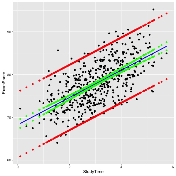
The curve in the confidence interval lines is clearly visible toward the extremes of the graph. The prediction interval is also curved, but the curvature is not obvious in the graph. The equations for the confidence interval are described next.
First, we need an appropriate error term, thus:

Here Sy.x indicates the standard deviation of the residuals, N is the number of complete observations, Xi is the value of an individual observation on the predictor variable, X-bar is the mean on that variable, and the term on the bottom right is the sum of squared deviations from the mean for the predictor. Recall that the variance of the mean is SD2/N, which is essentially what we get if we multiply the MSE by 1/N – the left part of what is under the radical. The right part is essentially an adjustment for the distance of the observation from the mean of the predictor. The greater the distance from the mean, the larger the term and thus the greater error and wider the confidence interval. The right-most term is the reason for the curve in the confidence interval edges for the regression line.
The equation for constructing the actual confidence interval is
![]()
Where Y’ indicates the predicted value of Y (the value of the regression line itself), and t represents the t distribution.
Analogous quantities for the prediction interval are shown next.
The error term for the prediction interval is:

The alert reader will have noticed that the equations for the error term for the confidence and prediction intervals are identical except that the value ‘1’ appears inside the bracket for the prediction interval. The ‘1’ is missing from the confidence interval. If you note that the MSE get multiplied by each of the elements inside the bracket, then it should be clear that the function of the ‘1’ is to include the variance of the residuals (that is, the unexplained individual differences) into the error term. For the mean (confidence interval) the variance shrinks by 1/N, but for the individual (prediction interval) the variance between people – uncertainty about individual differences - must be included along with uncertainty about the mean.
The formula for the prediction interval is the same as for the confidence interval except that we swap out the error term:
The interpretation of the confidence interval is that 95% of the time we construct such an interval, the population regression line will fall within it. In any given application, we don’t know whether the population line is contained, which is why intervals set up by frequentist statistics are difficult understand.
The interpretation of the prediction interval is that if we were to draw someone new at random from the population represented by the regression, 95% of the time we do so, that new observation will fall within the interval. This turns out to have the same interpretation as the interval containing 95% of the population values on average over infinite trials. If we were to rerun this an infinite number of times, we would expect that the interval would contain 95% of the observation on average. As you can see from the figure, most of the observations fall inside the red lines.
Review
Why is the confidence interval for an individual point wider than for the regression line?
The confidence interval for the point (prediction interval) is wider than the confidence interval for the line because the line is essentially the mean. The confidence interval for the mean shrinks as the sample size increases. The prediction interval, however, must contain the individual differences variance, which does not diminish as the sample size increases.
Why are the confidence intervals for regression lines curved instead of being straight lines?
The regression line must pass through the means of X and Y, much like the fulcrum of a see-saw. A slight change in the slope of the line will make almost no difference in prediction at the mean, but as the regression line moves from the mean to the extremes, small differences in slope become magnified, much like moving up and down on the see-saw. Thus, if we sample data and compute a regression line repeatedly to create a sampling distribution of the regression line, a graph of those lines would produce a curve that is most narrow at the population means and increasingly wide as we move away from the mean of X.
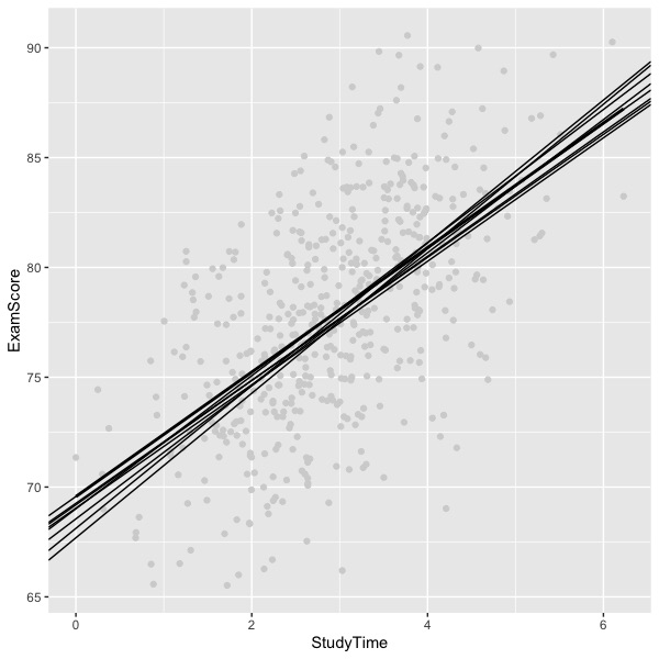
The figure below was created by repeatedly sampling 500 new people from the same population and computing the regression line on each sample. The figure shows nine such lines and thus begins to sketch an empirical sampling distribution of the regression line. As you can see, the lines approximate the same curved shape as shown by the confidence interval produced analytically using the formulas shown above. The shape of the population distribution of raw data is approximated by the light grey dots, which are only one sample of 500, not the entire population.
Shrinkage
The regression equation is fit so that the line of best fit minimizes the residual sum of squares and maximizes the variance accounted for (R-square). The method uses whatever data are observed in order to best fit the line. Doing so capitalizes on chance characteristics of the sample and results in an over-estimate of R-square for the population. In other words, the sample value of R-square is biased in that it is an over-estimate of the population value on average. Put another way, our obtained values of R-square based on raw data tend to be overly optimistic. The smaller the sample of data used to fit the line, the greater the opportunity for taking advantage of chance characteristics of the sample, and thus the greater the bias.
Given that we know the sample value is too large on average, is there a way we can estimate what R-square would be if we had the population? What if we were to take the regression equation and use it to make predictions on a new sample without re-estimating the equation? What might happen to R-square? In general, we expect R-square to reduce or to shrink from our initial sample value in such circumstances.
Conventional shrinkage formulas. If the population value of R2 is zero, then in the sample, the expected value of R2 is k/(N-1) where k is the number of predictors and N is the number of observations (typically people in psychological research).
In our hypothetical study of test scores and study time above, k is 1 and N is 500, so if it were true that R2 in the population was 0, then we would expect an observed R2 equal to 1/499 or .002, which is negligible. Although there does not appear to be a problem with capitalization on chance in our example, if you increase the number of predictors and reduce the number of observations, you can make R2 as large as you like. There is an ethical issue here because people tend to think that large values of R2 mean good quality predictions. Although that is often the case, it is no longer true when you have lots of predictors and few observations. The shrinkage formula applied by most statistical packages is
 ,
,
where the term on the left is the shrunken estimate. The equation shows that the estimated population value is a function of sample size, the number of predictors, and the initial value (sample estimate) of R2. A couple of examples may help make the formula for intuitive. Here we will assume that k = 4 predictors.
| N= | Adj R2 |
|---|---|
| 15 | .497 |
| 30 | .583 |
| 100 | .625 |
| N= | Adj R2 |
|---|---|
| 15 | .020 |
| 30 | .188 |
| 100 | .271 |
As you can see, the initial value of R2 matters, as does the number of observations. With four predictors and only 15 observations, R2 drops from a reasonable .3 to a negligible .02. With larger nunbers of predictors, shrinkage would be more severe, and with fewer predictors, less severe.
Running a regression program (R package lm) on a sample of data (N=500) from our early study of the effect of study time on exam scores yields the equation Y’ = 67.94 + 3.28StudyTime. The sample R2 is .3561 and the adjusted R2 is .3548, that is, 1-(1-.3561)*(500-1)/(500-1-1) = .3548. In the study time example, there is very little shrinkage. Most people consider it good form to present both the original and adjusted (shrunken) values of R2 in a report, particularly if there are several predictors and a small(ish) sample size. Also note that the shrinkage formula will not work properly if the analyst has tried a number of regression equations and selected a subset of predictors for the final model, particularly if that final model was chosen to maximize R2 . In such a case, the equation would underestimate the amount of shrinkage.
Cross-validation
Once a study is complete, the regression equation has been estimated and can be used on new cases to make predictions. That is, in the new sample, do not estimate the regression equation. Because the initial equation benefits by chance characteristics of the sample, we expect that the predictions won’t be quite as good when applied to new data. The process of checking on how good the predictions are in a new sample is called cross-validation. It’s quite simple: apply the equation as is (no re-estimation of the equation) to some new data, collect both predictions and outcomes for the new data, and compute the R2 for the new sample. Doing so does not capitalize on chance and estimates the operational predictive ability of the original equation. As with the shrinkage formula, we expect the cross validation R2 to be somewhat smaller in the new sample, depending on the number of predictors and the sample size of the initial study. In the case of cross-validation, however, the sample size for the second (cross-validation) study will impact the precision of the new R2 (larger sample result in more precise estimates).
In some contexts, true cross validation may be easy to complete. If people are routinely tested (e.g., college admissions) and the outcome variable(s) are routinely collected (e.g., freshman grade point average), then one year’s data might be used for deriving the regression and the second year’s data might be used for cross-validation. In other contexts, it may be difficult to collect sufficient data to carry out the cross-validation (people might be in short supply, the outcome variable might need to be measured specifically for the study, etc.). In the latter case, it is common for the researcher to split the data in the validation study into two random pieces, one of which serves as the validation sample, and the other of which serves as the cross-validation sample. That is, one can estimate the regression equation on one piece and apply the cross-validation to another. Computer programs can randomly split the data into such segments repeatedly (e.g. rerun the analysis ten times) and report a distribution of cross-validation R2 values along with the average result. Readers tend to find cross-validation reports as conservative, so if your cross-validation results show an R2 that is significant and large enough to be meaningful in your given context, this is persuasive evidence that the regression is actually useful.
Math estimates. Statisticians have worked out some estimates for cross-validation that are analogous to the shrinkage formula presented earlier. There are two: one for fixed-effects, and one for random-effects.
Fixed effects:


Random effects:

You won't see these formulas used much. If they have lots of data, people usually will run actual cross-validation analyses and report the results.
Review
What is shrinkage in the context of multiple regression? What are the things that affect the expected amount of shrinkage?
Shrinkage refers to the drop in R2 from the value estimated in the sample to either the population value or to a cross-validation value. The initial sample capitalizes on chance to result in an upwardly biased value of R2. The things that matter are the sample size, the number of predictors, and the size of R2.
What is cross-validation? Why is it important?
Cross-validation is the process of checking the operational predictive ability of a regression equation by applying the equation to new data without re-estimation of the regression coefficients. It is important because it yields a less biased assessment of the quality of prediction.
Predictor Selection
Predictor selection is the process of choosing a subset of independent variables to comprise a final regression model that represents one’s data. Let’s pause for a moment to recall that regression is used both for prediction explanation. Researchers often begin with a set of predictors that they feel are theoretically and/or practically relevant to the problem at hand. After running the regression, they often prune the equation by eliminating those predictors with nonsignificant slope estimates. Doing so results in a more parsimonious model, but may also result in serious misspecification, that is, the resulting model may not well represent the model that is true in the population. Such a misspecification is particularly likely when predictors are highly correlated because the power of tests for slopes will be reduced. If prediction is the sole interest, then choosing one of two highly correlated variables to retain makes sense – the second variable is largely redundant with the first and will add little predictive value. Choose whichever you like, it won’t matter much (you might choose based on cost of information). However, if explanation is the main goal, then eliminating one of the two highly correlated variables may be detrimental to our understanding of how things work.
In this section, we will work through a number of variable selection algorithms. These are programmed into the computer to choose the ‘best’ set of predictors for you. One of these (‘stepwise’) is very popular. You should never use any of these if your goal is explanation or understanding of phenomena of interest. Their purpose is efficiency – to provide the maximum R2 for the minimum number of predictors. In my opinion, their value is dubious, but you should know what they are so as to understand their drawbacks.
If you are going to choose some minimum number predictors for the maximum R2, the best approach is all possible regressions. You can instruct the computer to run all possible combinations of the predictors and sort the results by R2. An example presented by Pedhazur (1997) will be used to illustrate the methods.
| GPA | GREQ | GREV | MAT | AR | |
|---|---|---|---|---|---|
| GPA (Y) | 1 | ||||
| GREQ | .611 | 1 | |||
| GREV | .581 | .468 | 1 | ||
| MAT | .604 | .267 | .426 | 1 | |
| AR | .621 | .508 | .405 | .525 | 1 |
| Mean | 3.313 | 565.3 | 575.3 | 67.00 | 3.567 |
| SD | .600 | 48.61 | 83.03 | 9.248 | .838 |
The dependent variable in this example is graduate school grade point average. The tests (predictors) are the GRE verbal and quantitative scores, the Miller Analogies Test and a test of Arithmetic Reasoning. As you can see from the matrix shown above, the correlations among all the tests are moderate and positive. You can also see that each of the tests is correlated with the criterion, and nearly equally so. The GRE used to be normed to a mean of 500 and a standard deviation of 100. So if you are surprised by the sample values shown here, that’s why.
Let’s look at all possible regressions
| k | R2 | Variables in Model |
|---|---|---|
| 1 | .385 | AR |
| 1 | .384 | GREQ |
| 1 | .365 | MAT |
| 1 | .338 | GREV |
| 2 | .583 | GREQ MAT |
| 2 | .515 | GREV AR |
| 2 | .503 | GREQ AR |
| 2 | .493 | GREV MAT |
| 2 | .492 | MAT AR |
| 2 | .485 | GREQ GREV |
| 3 | .617 | GREQ GREV MAT |
| 3 | .610 | GREQ MAT AR |
| 3 | .572 | GREV MAT AR |
| 3 | .572 | GREQ GREV AR |
| 4 | .640 | GREQ GREV MAT AR |
As you can see, there are 4 predictors and these are listed at the top of the correlation matrxi table. The largest R2 for any single variable was for arithmetic reasoning test. This could be seen at a glance at the initial table because the correlation with GPA is largest for the AR test.
With 2 predictors, the best combination is GREQ and MAT. With 3 predictors, the best combination is GREQ, GREV and MAT. There is, of course, only one possible combination of all 4 predictors. With all possible regressions, it is easy to spot the largest R2 for each number of predictors. Notice, however, that the choice of predictors does not include cost. In the case of graduate school admissions the GREV and GREQ are bundled, so that if we have one, then we have the other. From the school’s perspective, the cost of testing might be considered minimal because the applicant pays for the test. However, the applicant may refuse to pay for some tests and thus refuse to apply to some schools, so there may be some hidden costs as well. In other contexts, the organization may pay for all the predictor measures, and thus some account might be taken of the relative costs involved. The algorithms described here do not account for costs.
Conventional algorithms for variable selection include forward, backward and stepwise. We will also mention blockwise, but it is not often used.
Forward selection proceeds by selecting the predictor with the largest criterion correlation that is significant according to the user’s specification (usually p.< 05 or p <.10). In our example, forward selection would first choose AR. It would then add the next predictor with the largest increment in R2, so long as the increment in R2 was significant (at the alpha set by the user). So in step 2 of our example, it would add GREV, increasing R2 from .385 to .515. Notice that this is not be best possible R2 for two variables. Next, forward would examine the remaining variables for inclusion. Let’s suppose that an R2 of .572 is not a significant increase from .515. If so, the algorithm would stop with the equation relating GPA to AR and GREV. Recall our earlier mention of the link between GREV and GREQ. If the R2 increase from .515 to .572 were significant, the algorithm would add GREQ to the model, and so forth. As you can see, forward selection does not necessarily result in the maximum R2 for a given number of variables. Although AR has the largest correlation with GPA, it is not part of the 2-variable model with the largest R2 for these data. The issue is that once a variable is included in the model, it never leaves, so that variables that ultimately become redundant with other predictors are never eliminated.
Backward selection is essentially the opposite of forward selection. Instead of starting empty and building up, the backward selection starts with the full model, and reduces it by eliminating variables one at a time. So backward would start with all 4 variables and an R2 of .64. It would then look to eliminate the variable with a non-significant, minimum loss of R2. So let’s say that the difference between R2 of .64 and .617 is not significant. Then AR would be eliminated. If none of the rest of the variables could be eliminated without significant reduction in R2, it would stop. Otherwise, it would look to eliminate GREV, leaving GREQ and MAT. Here again, there is a problem for maximizing R2. Variables that have been eliminated at one step are never considered again, so AR cannot make it back into the mix, even at the final step.
This leads to the most popular of the algorithms, stepwise. In stepwise, we start with forward selection, but at each step, we also consider whether any variables can be eliminated without significant loss (a sort of backwards check). So in our example, we would start by adding AR, which obviously cannot be eliminated without significant reduction in R2. In the second step, we add GREV, and then examine whether removing AR results in a significant decrement. If we lose R2 by removing AR, then we keep it. Otherwise, out it goes, and we look at adding the remaining variables. So at each step, we add whatever gives us the biggest increment after the variables already in the model, and also check to see if we can safely remove variables already in the model. Thus stepwise appears to address the problems of forward and backward solutions. But notice that stepwise is still not guaranteed to result in the model with the largest R2. If both AR and GREV show significant increments above each other, and it appears that they do in the current data, stepwise would not choose GREQ and MAT for the 2-variable model, even though this is the 2-variable combination with the highest R2. This is why all possible regressions is the best choice for choosing a model with the largest R2 for the fewest variables.
Blockwise starts by using forward selection by blocks of variables (e.g., personality tests in a block or group, ability tests in a block) and then any method, including stepwise, to choose variables within a block. Blockwise allows us to ignore large correlations within blocks at the initial stage. I do not recall seeing this method used.
The main idea in variable selection is efficiency – maximize R2 and minimize the number of predictors. But we want to minimize predictors because it takes resources to get the information – we must collect information or buy it somehow. (Some of the computer scraping algorithms appear to do this with minimal cost by roving the internet, but it remains to be seen how well these will work.) The selection algorithms do not account for the costs of information. If you really want to do predictor selextion, I suggest that you incorporate cost into the examination of all possible regressions so you can defend your final model as best in the sense of cost to benefit. If you are running a regression to test theoretical propositions or to better understand the process that results in the outcome of interest, avoid the selection algorithms.
Review
What are the main problems as far as R2 and prediction are concerned with forward (backward, stepwise, blockwise, all possible regressions)?
Of the algorithms, only using all possible regressions will always yield the maximum R2 for a given number of predictors. None of the algorithms considers the cost of information, that is, the cost of each predictor, which is important if your goal is efficient prediction.
Hierarchical Regression
Hierarchical regression refers to pre-planned tests of significance for one or more predictors in a regression equation. Although it looks similar to the selection algorithms, it is different in that any tests are planned before the data are collected. This is the approach to use when understanding or theory testing is the main goal of the analysis.
Example of application. Suppose we want to know whether personality tests increase prediction of medical school success beyond that afforded by cognitive ability tests. We already use cognitive ability in our selection process (the MCAT), but we are considering adding a personality test to our admissions process. We have about 250 medical students enrolled in the first two years of medical school. We have their MCAT scores on file, and we have given each of them a personality test (a so-called ‘Big Five’ measures that yields scores on openness to experience, conscientiousness, extroversion, agreeableness and neuroticism). Further suppose that, based on the research literature, we think that the conscientiousness and neuroticism measures will add predictive ability, so those are the only personality measures we will include in our study.
Suppose that we collect data on 250 med students in their first two years (data are hypothetical). Our first model considers only the cognitive ability test and undergraduate GPA (the status quo for the current selection system):
MedGPA = a + b1UgGPA + b2MCAT. We find that R2 = .10, p <.05.
This is our baseline model. We want to know if adding our personality measures will significantly add to the predictive ability of the model. Thus our second model is
MedGPA = a + b1UgGPA + b2MCAT + b3Conscientious + b4Neuroticism. We find R2 = .13, p <.05.
The hierarchical test is whether the addition of the two new variables increases R2 significantly. The form of the test is:

Where the subscripts L and S refer to the models with larger and smaller number of predictors. The result of the test is
F(2,245)=4.22, p < .05
So in this case, we can say that the addition of personality tests significantly increases the value of R2. That is, we get better predictive ability by including the two personality scales. This test does not address the significance of the regression coefficients for conscientiousness and neuroticism, which may or may not be statistically significant individually. It does directly address the research question of interest, which was whether the hypothesized set of personality scales would improve prediction.
Hierarchical regression is typically used when the research question has a theoretical underpinning. Usually this kind of test is reported in research articles.
Review
What is the main conceptual difference between the variable selection algorithms and hierarchical regression?
The main difference is one of a planned comparison (hierarchical) vs letting the data decide on a final model (selection algorithms). Both consider the predictive ability of regression models.
References
Pedhazur, E. J. (1997). Multiple regression in behavioral research. Fort Worth, TX: Harcourt Brace.