Questions

Write a raw score regression equation with 2 ivs in it.

What is the difference in interpretation of b weights in simple regression vs. multiple regression?

Describe R-square in two different ways, that is, using two distinct formulas. Explain the formulas.

What happens to b weights if we add new variables to the regression equation that are highly correlated with ones already in the equation?

Why do we report beta weights (standardized b weights)?

Write a regression equation with beta weights in it.

What are the three factors that influence the standard error of the b weight?

How is it possible to have a significant R-square and non-significant b weights?

The Regression Line

With one independent variable, we may write the regression equation as:

Where Y is an observed score on the dependent variable, a is the intercept, b is the slope, X is the observed score on the independent variable, and e is an error or residual.

We can extend this to any number of independent variables:

(3.1)

Note that we have k independent variables and a slope for each. We still have one error and one intercept. Again we want to choose the estimates of a and b so as to minimize the sum of squared errors of prediction. The prediction equation is:

(3.2)

Finding the values of b (the slopes) is tricky for k>2 independent variables, and you really need matrix algebra to see the computations. It's simpler for k=2 IVs, which we will discuss here. But the basic ideas are the same no matter how many independent variables you have. If you understand the meaning of the slopes with two independent variables, you will likely be good no matter how many you have.

For the one variable case, the calculation of b and a was:

For the two variable case:

and

At this point, you should notice that all the terms from the one variable case appear in the two variable case. In the two variable case, the other X variable also appears in the equation. For example, X₂ appears in the equation for b₁. Note that terms corresponding to the variance of both X variables occur in the slopes. Also note that a term corresponding to the covariance of X1 and X2 (sum of deviation cross-products) also appears in the formula for the slope.

The equation for a with two independent variables is:

This equation is a straight-forward generalization of the case for one independent variable.

A Numerical Example

Suppose we want to predict job performance of Chevy mechanics based on mechanical aptitude test scores and test scores from personality test that measures conscientiousness. (In practice, we would need many more people, but I wanted to fit this on a PowerPoint slide.)

Job Perf	Mech Apt	Consc
Y	X1	X2	X1*Y	X2*Y	X1*X2
1	40	25	40	25	1000
2	45	20	90	40	900
1	38	30	38	30	1140
3	50	30	150	90	1500
2	48	28	96	56	1344
3	55	30	165	90	1650
3	53	34	159	102	1802
4	55	36	220	144	1980
4	58	32	232	128	1856
3	40	34	120	102	1360
5	55	38	275	190	2090
3	48	28	144	84	1344
3	45	30	135	90	1350
2	55	36	110	72	1980
4	60	34	240	136	2040
5	60	38	300	190	2280
5	60	42	300	210	2520
5	65	38	325	190	2470
4	50	34	200	136	1700
3	58	38	174	114	2204
Y	X1	X2	X1*Y	X2*Y	X1*X2
65	1038	655	3513	2219	34510	Sum
20	20	20	20	20	20	N
3.25	51.9	32.75	175.65	110.95	1725.5	M
1.25	7.58	5.24	84.33	54.73	474.60	SD
29.75	1091.8	521.75				USS

We can collect the data into a matrix like this:

	y	X1	X2
Y	29.75	139.5	90.25
X1	0.77	1091.8	515.5
X2	0.72	0.68	521.75

 

The numbers in the table above correspond to the following sums of squares, cross products, and correlations:

	y	x1	X2
Y
X1
X2

We can now compute the regression coefficients:

To find the intercept, we have:

Therefore, our regression equation is:

Y '= -4.10+.09X1+.09X2 or

Job Perf' = -4.10 +.09MechApt +.09Coscientiousness.

Visual Representations of the Regression

We have 3 variables, so we have 3 scatterplots that show their relations.

 

Because we have computed the regression equation, we can also view a plot of Y' vs. Y, or actual vs. predicted Y.

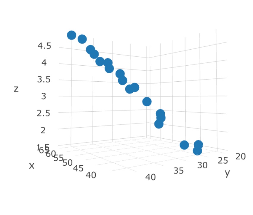
We can (sort of) view the plot in 3D space, where the two predictors are the X and Y axes, and the Z axis is the criterion, thus:

This graph doesn't show it very well, but the regression problem can be thought of as a sort of response surface problem. What is the expected height (Z) at each value of X and Y? An example animation is shown at the very top of this page (rotating figure). The linear regression solution to this problem in this dimensionality is a plane. The plotly package in R will let you 'grab' the 3 dimensional graph and rotate it with your computer mouse. This lets you see the response surface more clearly. A still view of the Chevy mechanics' predicted scores produced by Plotly:

R-square (R²)

Just as in simple regression, the dependent variable is thought of as a linear part and an error. In multiple regression, the linear part has more than one X variable associated with it. When we run a multiple regression, we can compute the proportion of variance due to the regression (the set of independent variables considered together). This proportion is called R-square. We use a capital R to show that it's a multiple R instead of a single variable r. We can also compute the correlation between Y and Y' and square that. If we do, we will also find R-square.

 

Y	X1	X2	Y'	Resid
2	45	20	1.54	0.46
1	38	30	1.81	-0.81
3	50	30	2.84	0.16
2	48	28	2.50	-0.50
3	55	30	3.28	-0.28
3	53	34	3.45	-0.45
4	55	36	3.80	0.20
4	58	32	3.71	0.29
3	40	34	2.33	0.67
5	55	38	3.98	1.02
3	48	28	2.50	0.50
3	45	30	2.41	0.59
2	55	36	3.80	-1.80
4	60	34	4.06	-0.06
5	60	38	4.41	0.59
5	60	42	4.76	0.24
5	65	38	4.84	0.16
4	50	34	3.19	0.80
3	58	38	4.24	-1.24
M = 3.25	51.9	32.75	3.25	0
V = 1.57	57.46	27.46	1.05	0.52
USS=29.83			19.95	9.88

The mean of Y is 3.25 and so is the mean of Y'. The mean of the residuals is 0. The variance of Y is 1.57. The variance of Y' is 1.05, and the variance of the residuals is .52. Together, the variance of regression (Y') and the variance of error (e) add up to the variance of Y (1.57 = 1.05+.52). R-square is 1.05/1.57 or .67. If we compute the correlation between Y and Y' we find that R=.82, which when squared is also an R-square of .67. (Recall the scatterplot of Y and Y'). R-square is the proportion of variance in Y due to the multiple regression.

Testing the Significance of R²

You have already seen this once, but here it is again in a new context:

which is distributed as F with k and (N-k-1) degrees of freedom when the null hypothesis (that R-square is zero in the population) is true. Now R² represents the multiple correlation rather than the single correlation that we saw in simple regression. For our most recent example, we have 2 independent variables, an R² of .67, and 20 people, so

p < .01. (F_crit for alpha = .01 is about 6).

Because SStot=SSreg+SSres , we can compute an equivalent F using sums of squares and associated df.

which agrees with our earlier result within rounding error.

Standardized & Unstandardized Weights

Each X variable will have associated with it one slope or regression weight. Each weight is interpreted as the unit change in Y given a unit change in X, holding the other X variables constant. If we want to make point predictions (predictions of the actual value of the dependent variable) given values of the independent variables, these are the weights we want. For example, if we have undergraduate grade point average and SAT scores for a person and want to predict their college freshman GPA, the unstandardized regression weights do the job.

Variables with large b weights ought to tell us that they are more important because Y changes more rapidly for some of them than for others. The problem with unstandardized or raw score b weights in this regard is that they have different units of measurement, and thus different standard deviations. If we measured X = height in feet rather than X = height in inches, the b weight for feet would be 12 times larger than the b for inches (12 inches in a foot; in both cases we interpret b as the unit change in Y when X changes 1 unit). So when we measure different X variables in different units, part of the size of b is attributable to units of measurement rather than importance per se. So what we can do is to standardize all the variables (both X and Y, each X in turn). If we do that, then all the variables will have a standard deivation equal to one, and the connecton to the X variables will be readily apparent by the size of the b weights -- all will be interpreted as the number of standard deviations that Y changes when each X changes one standard deviation. The standardized slopes are called beta weights. This is an extremely poor choice of words and symbols, because we have already used beta to mean the population value of b (don't blame me; this is part of the literature). Generally speaking, in multiple regression, beta will refer to standardized regression weights, that is, to estimates of parameters, unless otherwise noted.

Regression Equations with beta weights

Because we are using standardized scores, we are back into the z-score situation. As you recall from the comparison of correlation and regression:

But beta means a b weight when X and Y are in standard scores, so for the simple regression case, r = beta, and we have:

The earlier formulas I gave for b were composed of sums of square and cross-products .

But with z scores, we will be dealing with standardized sums of squares and cross-products. A standardized averaged sum of squares is 1

and a standardized averaged sum of cross products is a correlation coefficient

Bottom line on this is we can estimate beta weights using a correlation matrix. With simple regression, as you have already seen, r=beta . With two independent variables,

and

where r_y1 is the correlation of y with X1, r_y2 is the correlation of y with X2, and r₁₂ is the correlation of X1 with X2. Note that the two formulas are nearly identical, the exception is the ordering of the first two symbols in the numerator.

Our correlation matrix looks like this:

	Y	X1	X2
Y	1
X1	0.77	1
X2	0.72	0.68	1

Note that there is a surprisingly large difference in beta weights given the magnitude of correlations.

Let's look at this for a minute, first at the equation for beta₁. The numerator says that beta₁ is the correlation (of X₁ and Y) minus the correlation (of X₂ and Y) times the predictor correlation (X₁ and X₂). The denominator says boost the numerator a bit depending on the size of the correlation between X₁ and X₂. Suppose r₁₂ is zero. Then r_y2r₁₂ is zero, and the numerator is r_y1. The denominator is 1, so the result is r_y1, the simple correlation between X₁ and Y. If the correlation between X₁ and X₂ is zero, the beta weight is the simple correlation. On the other hand, if the correlation between X₁ and X₂ is 1.0, the beta is undefined, because we would be dividing by zero. So our life is less complicated if the correlation between the X variables is zero.

Calculating R²

As I already mentioned, one way to compute R² is to compute the correlation between Y and Y', and square that. There are some other ways to calculate R², however, and these are important for a conceptual understanding of what is happening in multiple regression. If the independent variables are uncorrelated, then

This says that R², the proportion of variance in the dependent variable accounted for by both the independent variables, is equal to the sum of the squared correlations of the independent variables with Y. This is only true when the IVs are orthogonal (uncorrelated).

In our example, R² is .67. The correlations are r_y1=.77 and r_y2 = .72. If we square and add, we get .77²+.72² = .5929+.5184 = 1.11, which is clearly too large a value for R², which is bounded by zero and one.

If the IVs are correlated, then we have some shared X and possibly shared Y as well, and we have to take that into account. Two general formulas can be used to calculate R² when the IVs are correlated.

This says to multiply the standardized slope (beta weight) by the correlation for each independent variable and add to calculate R². What this does is to include both the correlation, (which will overestimate the total R² because of shared Y) and the beta weight (which underestimates R² because it only includes the unique Y and discounts the shared Y). Appropriately combined, they yield the correct R². Note that when r₁₂ is zero, then beta₁ = r_y1 and beta₂ = r_y2, so that (beta₁)( r_y1 )= r²_y1 and we have the earlier formula where R² is the sum of the squared correlations between the Xs and Y. For our example, the relevant numbers are (.52).77+(.37).72 = .40+.27 = .67, which agrees with our earlier value of R².

 A second formula using only correlation coefficients is

This formula says that R² is the sum of the squared correlations between the Xs and Y adjusted for the shared X and shared Y. Note that the term on the right in the numerator and the variable in the denominator both contain r₁₂, which is the correlation between X1 and X2. Note that this equation also simplifies the simple sum of the squared correlations when r₁₂ = 0, that is, when the IVs are orthogonal. For our example, we have

which is the same as our earlier value within rounding error.

 

Tests of Regression Coefficients

Each regression coefficient is a slope estimate. With more than one independent variable, the slopes refer to the expected change in Y when X changes 1 unit, CONTROLLING FOR THE OTHER X VARIABLES. That is, b₁ is the change in Y given a unit change in X₁ while holding X₂ constant, and b₂ is the change in Y given a unit change in X₂ while holding X₁ constant. We will develop this more formally after we introduce partial correlation. We would like to test whether the slope (b) has some value, typically, whether the slope is zero in the population. To do that, we will compare the value of b to its standard error, similar to what we did for the t-test, where we compared the differnce in means to its standard error.

The standard error of the b weight for the two variable problem:

where s²_y.12 is the variance of estimate (the variance of the residuals). The standard error of the b weight depends upon three things. The variance of estimate tells us about how far the points fall from the regression line (the average squared distance). Large errors in prediction mean a larger standard error. The sum of squares of the IV also matter. The larger the sum of squares (variance) of X, the smaller the standard error. Restriction of range not only reduces the size of the correlation, but also increases the standard error of the b weight. The correlation between the independent variables also matters. The larger the correlation, the larger the standard error of the b weight. So to find significant b weights, we want to minimize the correlation between the predictors, maximize the variance of the predictors, and minimize the errors of prediction.

Consider these when you are designing your research. If you don't you could have a problem with power for the significance test, and your hard work may not pay off. Domains where prediction is poor will be harder to show relations (obviously, but this is where the variance of residuals comes from). If you are selecting people for the study, make sure that the vary widely on the predictors. If you do research on volunteers at a highly selective university, you will have a restricted range of cognitive ability, so it will be harder to show a significant regression weight for a test of cognitive ability. Pick the predictors with care - if they are highly corrrelated, you can have a significant R-square but nonsignificant regression weights. You may have noticed that sample size is not explictly incorporated in the formula. However, the sum of squares for the independent variable is included, and this will increase the denominator as sample size increases, thus decreasing the standard error. So larger sample sizes will result in better power as usual.

The variance of prediction is

and the test of the b weight is a t-test with N-k-1 degrees of freedom.

In our example, the sum of squared errors is 9.79, and the df are 20-2-1 or 17. Therefore, our variance of estimate is

.575871 or .58 after rounding. Our standard errors are:

and S_b2 = .0455, which follows from calculations that are identical except for the value of the sum of squares for X₂ instead of X₁.

To test the b weights for significance, we compute a t statistic

.

In our case, t = .0864/.0313 or 2.75. If we compare this to the t distribution with 17 df, we find that it is significant (from a lookup function, we find that p = .0137, which is less than .05).

For b₂, we compute t = .0876/.0455 = 1.926, which has a p value of .0710, which is not significant. Note that the correlation r_y2 is .72, which is highly significant (p < .01) but b₂ is not significant.

Tests of R² vs. Tests of b

Because the b-weights are slopes for the unique parts of Y (that is, the part of Y that can be attributed uniquely to the particular X in the regression equation) and because correlations among the independent variables increase the standard errors of the b weights, it is possible to have a large, significant R², but at the same time to have nonsignificant b weights (as in our Chevy mechanics example). It is also possible to find a significant b weight without a significant R². This can happen when we have lots of independent variables (usually more than 2), all or most of which have rather low correlations with Y. If one of these variables has a large correlation with Y, R² may not be significant because with such a large number of IVs we would expect to see as large an R² just by chance. If R² is not significant, you should usually avoid interpreting b weights that are significant. In such cases, it is likely that the significant b weight is a Type I error.

Testing Incremental R²

We can test the change in R² that occurs when we add a new variable to a regression equation. We can start with 1 variable and compute an R² (or r²) for that variable. We can then add a second variable and compute R² with both variables in it. The second R² will always be equal to or greater than the first R². If it is greater, we can ask whether it is significantly greater. To do so, we compute

where R²_L is the larger R² (with more predictors), k_L is the number of predictors in the larger equation and k_S is the number of predictors in the smaller equation. When the null is true, the result is distributed as F with degrees of freedom equal to (k_L - k_S) and (N- k_L -1). In our example, we know that R²_y.12 = .67 (from earlier calculations) and also that r_y1 = .77 and r_y2 = .72. r²_y1=.59 and r²_y2=.52. Now we can see if the increase of adding either X1 or X2 to the equation containing the other increases R² to significant extent. To see if X1 adds variance we start with X2 in the equation:

Our critical value of F(1,17) is 4.45, so our F for the increment of X1 over X2 is significant.

For the increment of X2 over X1, we have

Our critical value of F has not changed, so the increment to R² by X2 is not (quite) significant.