Regression Basics
Questions
What are predictors and criteria?
According to the regression (linear) model, what are the two parts of variance of the dependent variable? (Write an equation and state in your own words what this says.)
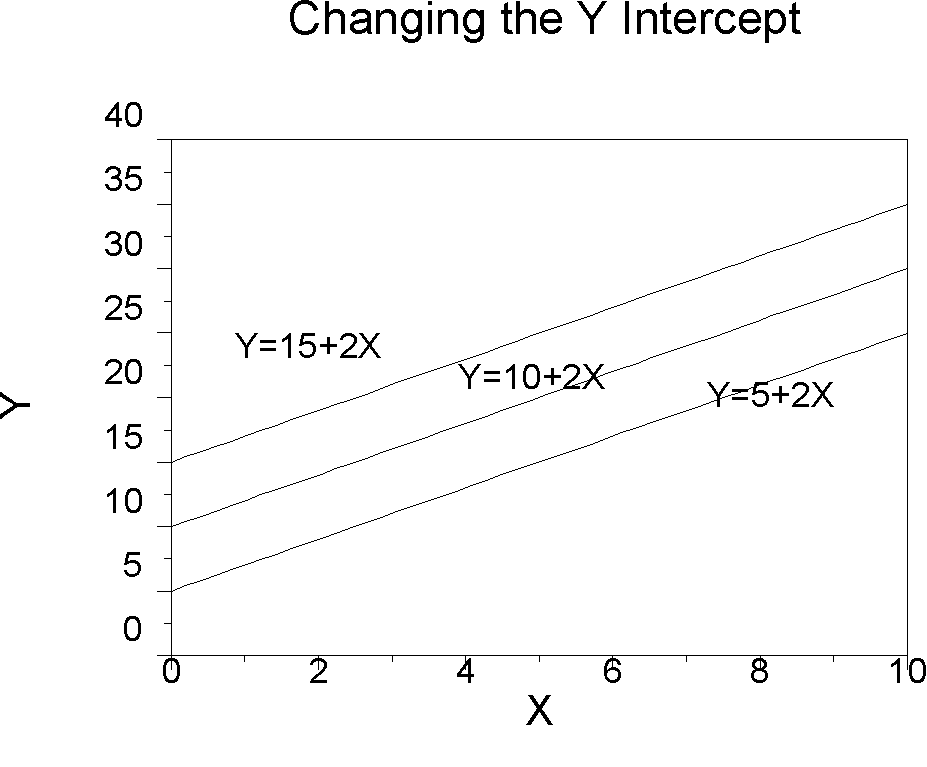
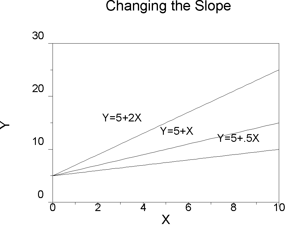
How do changes in the slope and intercept affect (move) the regression line?
What does it mean to choose a regression line to satisfy the loss function of least squares?
How do we find the slope and intercept for the regression line with a single independent variable? (Either formula for the slope is acceptable.)
What does it mean to test the significance of the regression sum of squares? R-square?
Why does testing for the regression sum of squares turn out to have the same result as testing for R-square?
The Linear Model
The linear model assumes that the relations between two variables can be summarized by a straight line.
|
Jargon. It is customary to call the independent variable X and the dependent variable Y. The X variable is often called the predictor and Y is often called the criterion (the plural of 'criterion' is 'criteria'). It is customary to talk about the regression of Y on X, so that if we were predicting GPA from SAT we would talk about the regression of GPA on SAT. |
Scores on a dependent variable can be thought of as the sum of two parts: (1) a linear function of an independent variable, and (2) random error. In symbols, we have:
![]() (2.1)
(2.1)
Where Yi is a score on the dependent variable for the ith person, a + b Xi describes a line or linear function relating X to Y, and e i is an error. Note that there is a separate score for each X, Y, and error (these are variables), but only one value of a (alpha) and b (beta) , which are population parameters.
The portion of the equation denoted by a + b Xi defines a line. The symbol X represents the independent variable. The symbol a represents the Y intercept, that is, the value that Y takes when X is zero. The symbol b describes the slope of a line. It denotes the number of units that Y changes when X changes 1 unit. If the slope is 2, then when X increases 1 unit, Y increases 2 units. If the slope is -.25, then as X increases 1 unit, Y decreases .25 units. Equation 2.1 is expressed as parameters. We usually have to estimate the parameters.
The equation for estimates rather than parameters is:
![]() (2.2)
(2.2)
If we take out the error part of equation 2.2, we have a straight line that we can use to predict values of Y from values of X, which is one of the main uses of regression. It looks like this:
![]() (2.3)
(2.3)
Equation 2.3 says that the predicted value of Y is equal to a linear function of X. The slope of a line (b) is sometimes defined as rise over run. If Y is the vertical axis, then rise refers to change in Y. If X is the horizontal axis, then run refers to change in X. Therefore, rise over run is the ratio of change in Y to change in X. This means exactly the same thing as the number of units that Y changes when X changes 1 unit (e.g., 2/1 = 2, 10/12 = .833, -5/20=-.25). Slope means rise over run.
Linear Transformation
The idea of a linear transformation is that one variable is mapped onto another in a 1-to-1 fashion. A linear transformation allows you to multiply (or divide) the original variable and then to add (or subtract) a constant. In junior high school, you were probably shown the transformation Y = mX+b, but we use Y = a+bX instead. A linear transformation is what is permissible in the transformation of interval scale data in Steven's taxonomy (nominal, ordinal, interval, and ratio). The value a, the Y intercept, shifts the line up or down the Y-axis. The value of b, the slope, controls how quickly the line rises as we move from left to right.
|
|
|
One further example may help to illustrate the notion of the linear transformation. We can convert temperature in degrees Centigrade to degrees Fahrenheit using a linear transformation.
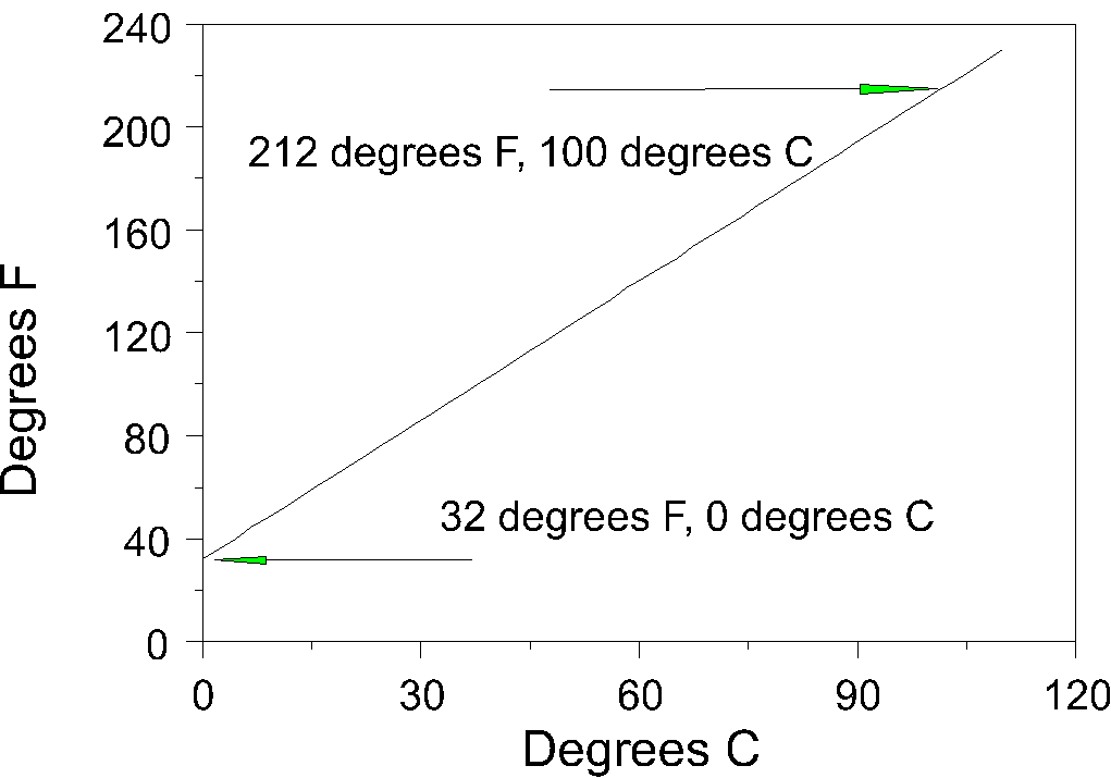
Note that the Y intercept is 32, because when X=0, Y=32. The slope is rise over run. Run is degrees C, or zero to 100 or 100. Rise over the same part of the line is 212-32, or 180. Therefore slope is 180/100 or 1.8. We can write the equation for the linear transformation Y'=32+1.8X or F=32+1.8C.
Simple Regression Example
The regression problems that we deal with will use a line to transform values of X to predict values of Y. In general, not all of the points will fall on the line, but we will choose our regression line so as to best summarize the relations between X and Y (best in this context will be defined shortly).
Suppose we measured the height and weight of a random sample of adults in shopping malls in the U.S. We want to predict weight from height in the population.
Table 2.1
|
Ht |
Wt |
|
|
61 |
105 |
|
|
62 |
120 |
|
|
63 |
120 |
|
|
65 |
160 |
|
|
65 |
120 |
|
|
68 |
145 |
|
|
69 |
175 |
|
|
70 |
160 |
|
|
72 |
185 |
|
|
75 N=10 |
210 N=10 |
|
|
67 |
150 |
Mean |
|
20.89 |
1155.5 |
Variance (S2) |
|
4.57 |
33.99 |
Standard Deviation (S) |
|
|
|
Correlation (r) = .94 |
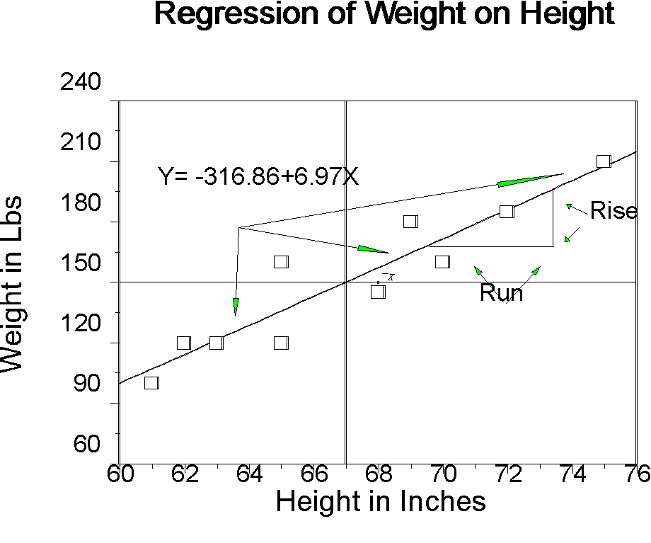
It is customary to talk about the regression of Y on X, hence the regression of weight on height in our example. The regression equation of our example is Y' = -316.86 + 6.97X, where -361.86 is the intercept (a) and 6.97 is the slope (b). We could also write that predicted weight is -316.86+6.97height. The slope value means that for each inch we increase in height, we expect to increase approximately 7 pounds in weight (increase does not mean change in height or weight within a person, rather it means change in people who have a certain height or weight). The intercept is the value of Y that we expect when X is zero. So if we had a person 0 inches tall, they should weigh -316.86 pounds. Of course we do not find people who are zero inches tall and we do not find people with negative weight. It is often the case in psychology the value of the intercept has no meaningful interpretation. Other examples include SAT scores, personality test scores, and many individual difference variables as independent variables. Occasionally, however, the intercept does have meaning. Our independent variable might be digits recalled correctly, number of siblings, or some other independent variable defined so that zero has meaning.
The linear model revisited. Remember that the linear model says each observed Y is composed of two parts, (1) a linear function of X, and (2) an error. We can illustrate this with our example.
Figure 2
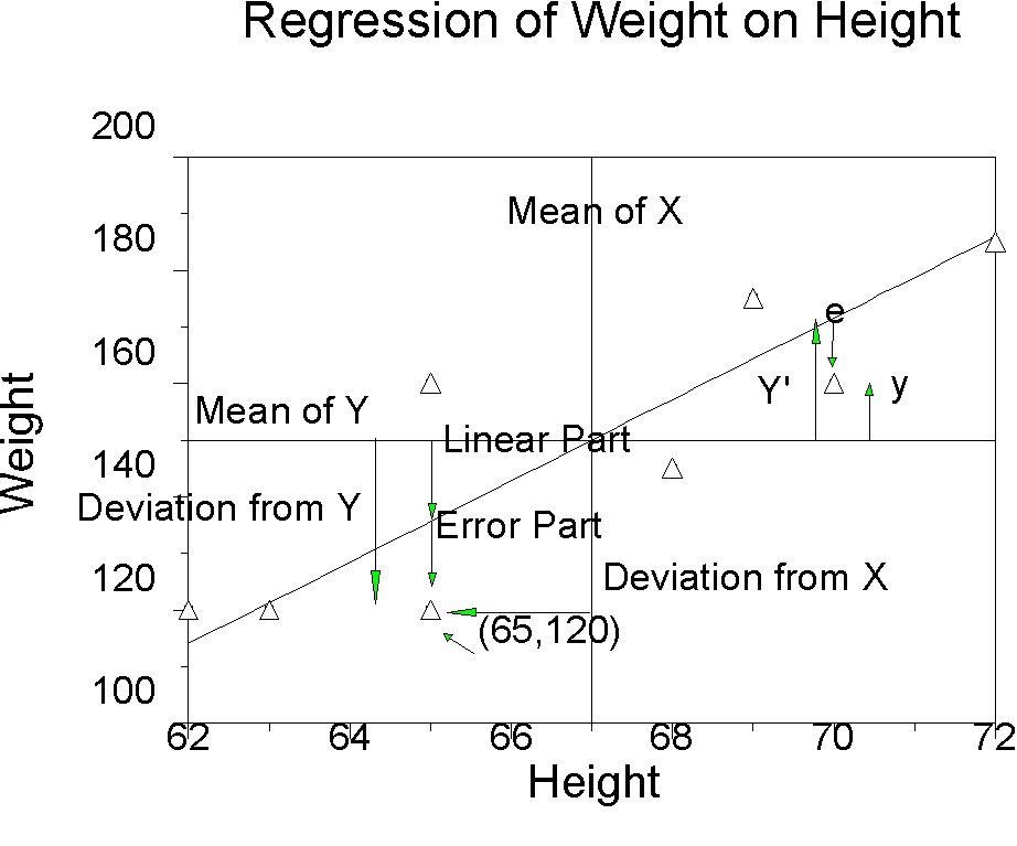
We can use the regression line to predict values of Y given values of X. For any given value of X, we go straight up to the line, and then move horizontally to the left to find the value of Y. The predicted value of Y is called the predicted value of Y, and is denoted Y'. The difference between the observed Y and the predicted Y (Y-Y') is called a residual. The predicted Y part is the linear part. The residual is the error.
Table 2
|
N |
Ht |
Wt |
Y' |
Resid |
|
1 |
61 |
105 |
108.19 |
-3.19 |
|
2 |
62 |
120 |
115.16 |
4.84 |
|
3 |
63 |
120 |
122.13 |
-2.13 |
|
4 |
65 |
160 |
136.06 |
23.94 |
|
5 |
65 |
120 |
136.06 |
-16.06 |
|
6 |
68 |
145 |
156.97 |
-11.97 |
|
7 |
69 |
175 |
163.94 |
11.06 |
|
8 |
70 |
160 |
170.91 |
-10.91 |
|
9 |
72 |
185 |
184.84 |
0.16 |
|
10 |
75 |
210 |
205.75 |
4.25 |
|
Mean |
67 |
150 |
150.00 |
0.00 |
|
Standard Deviation |
4.57 |
33.99 |
31.85 |
11.89 |
|
Variance |
20.89 |
1155.56 |
1014.37 |
141.32 |
Compare the numbers in the table for person 5 (height = 65, weight=120) to the same person on the graph. The regression line for X=65 is 136.06. The difference between the mean of Y and 136.06 is the part of Y due to the linear function of X. The difference between the line and Y is -16.06. This is the error part of Y, the residual. A couple of other things to note about Table 2.2 that we will come back to:
- The mean of the predicted values (Y') is equal to the mean of actual values (Y), and the mean of the residual values (e) is equal to zero.
- The variance of Y is equal to the variance of predicted values plus the variance of the residuals.
Placing the Regression Line
What are the values of the slope and intercept?
Finding the regression line: Method 1
It turns out that the correlation coefficient, r, is the slope of the regression line when both X and Y are expressed as z scores. Remember that r is the average of cross products, that is,
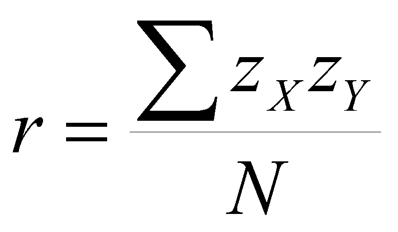
The correlation coefficient is the slope of Y on X in z-score form, and we already know how to find it. Just find the z scores for each variable, multiply them, and find the average. The correlation coefficient tells us how many standard deviations that Y changes when X changes 1 standard deviation. When there is no correlation (r = 0), Y changes zero standard deviations when X changes 1 SD. When r is 1, then Y changes 1 SD when X changes 1 SD.
The regression b weight is expressed in raw score units rather than z score units. To move from the correlation coefficient to the regression coefficient, we can simply transform the units:
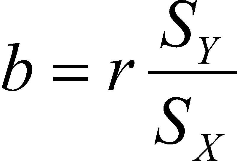 (2.4)
(2.4)
This says that the regression weight is equal to the correlation times the standard deviation of Y divided by the standard deviation of X. Note that r shows the slope in z score form, that is, when both standard deviations are 1.0, so their ratio is 1.0. But we want to know the number of raw score units that Y changes and the number that X changes. So to get new ratio, we multiply by the standard deviation of Y and divide by the standard deviation of X, that is, multiply r by the raw score ratio of standard deviations.
To find the intercept, a, we compute the following:
![]() (2.5)
(2.5)
This says take the mean of Y and subtract the slope times the mean of X. Now it turns out that the regression line always passes through the mean of X and the mean of Y.
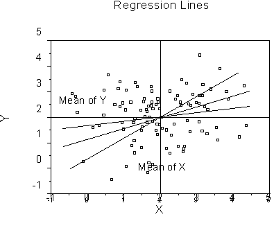
If there is no relationship between X and Y, the best guess for all values of X is the mean of Y. If there is a relationship (b is not zero), the best guess for the mean of X is still the mean of Y, and as X departs from the mean, so does Y. At any rate, the regression line always passes through the means of X and Y. This means that, regardless of the value of the slope, when X is at its mean, so is Y. We can write this as (from equation 2.3):
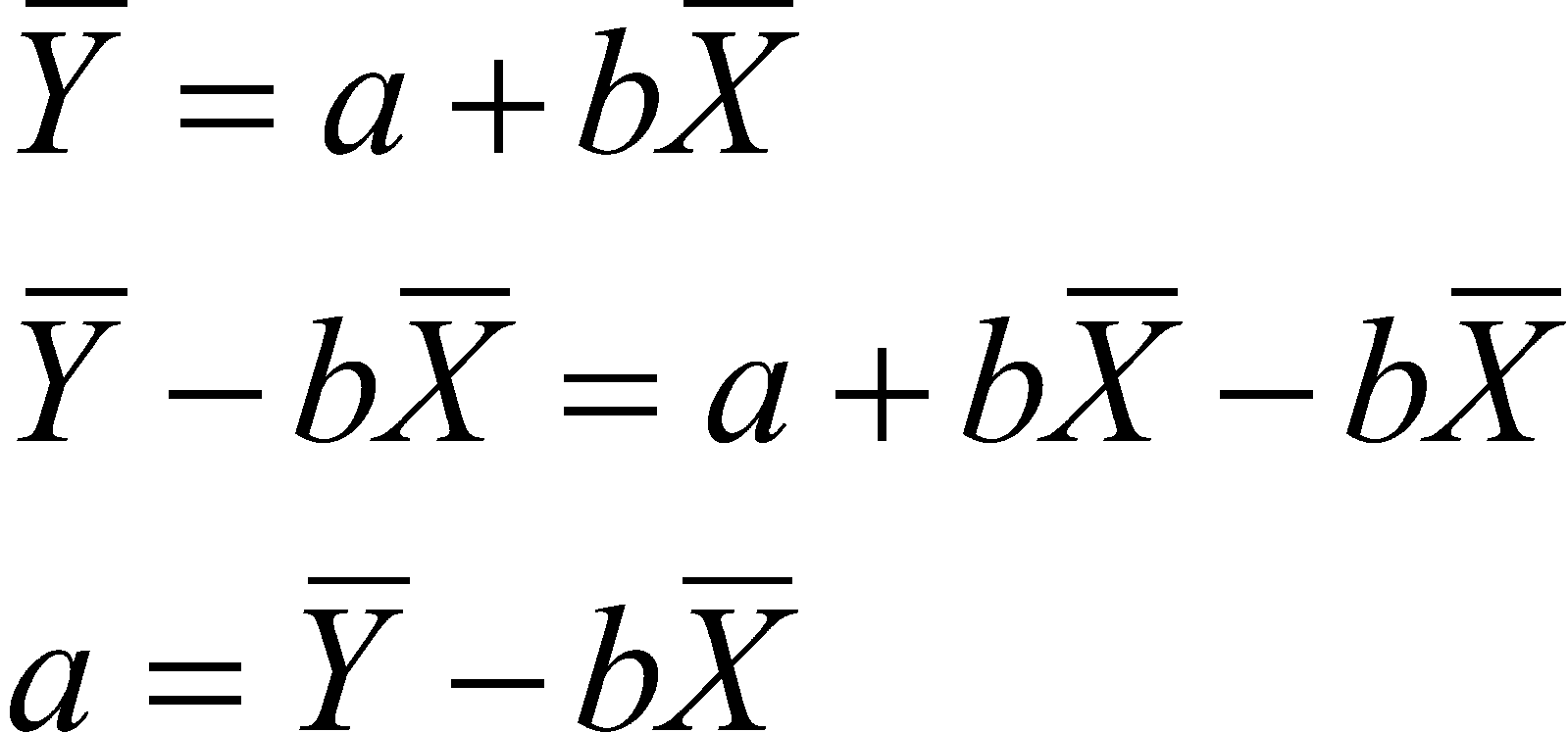
So just subtract and rearrange to find the intercept. Another way to think about this is that we know one point for the line, which is (![]() ). We also know the slope, so we can draw in the line until it crosses the Y-axis, that is, follow the line until X=0.
). We also know the slope, so we can draw in the line until it crosses the Y-axis, that is, follow the line until X=0.
We can rewrite the regression equation:
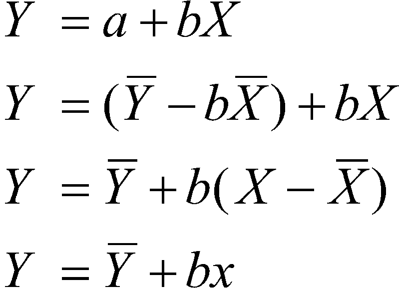
This interpretation of the regression line says start with the mean of Y, and slide up or down the regression line b times the deviation of X. For example, look back at Figure 2. Look for the deviation of X from the mean. Note the similarity to ANOVA, where you have a grand mean and each factor in the model is in terms of deviations from that mean.
Finding the regression line: Method 2
To find the slope, Pedhazur uses the formula:
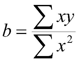 (2.6)
(2.6)
This yields the same result as I gave you in 2.5. To see why this is so, we can start with the formula I gave you for the slope and work down:
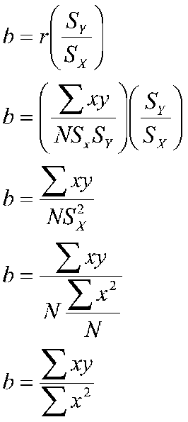
This says that the slope is the sum of deviation cross products divided by the sum of squares for X. Of course, this is the same as the correlation coefficient multiplied by the ratio of the two standard deviations.
Finding the regression line: The notion of least squares.
What we are about with regression is predicting a value of Y given a value of X. There are many ways we could do this (in actuarial prediction, used by insurance companies, you find whatever happened in the past and guess that it will happen in the future, e.g., what is the likelihood that a 21 year old male will crash his Neon?). However, the usual method that we use is to assume that there are linear relations between the two variables. If this is true, then the relations between the two can be summarized with a line. The question now is where to put the line so that we get the best prediction, whatever 'best' means. The statistician's solution to what 'best' means is called least squares. We define a residual to be the difference between the actual value and the predicted value (e = Y-Y'). It seems reasonable that we would like to make the residuals as small as possible, and earlier in our example, you saw that the mean of the residuals was zero. The criterion of least squares defines 'best' to mean that the sum of e2 is a small as possible, that is the smallest sum of squared errors, or least squares. It turns out that the regression line with the choice of a and b I have described has the property that the sum of squared errors is minimum for any line chosen to predict Y from X.
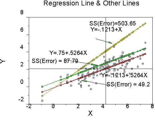
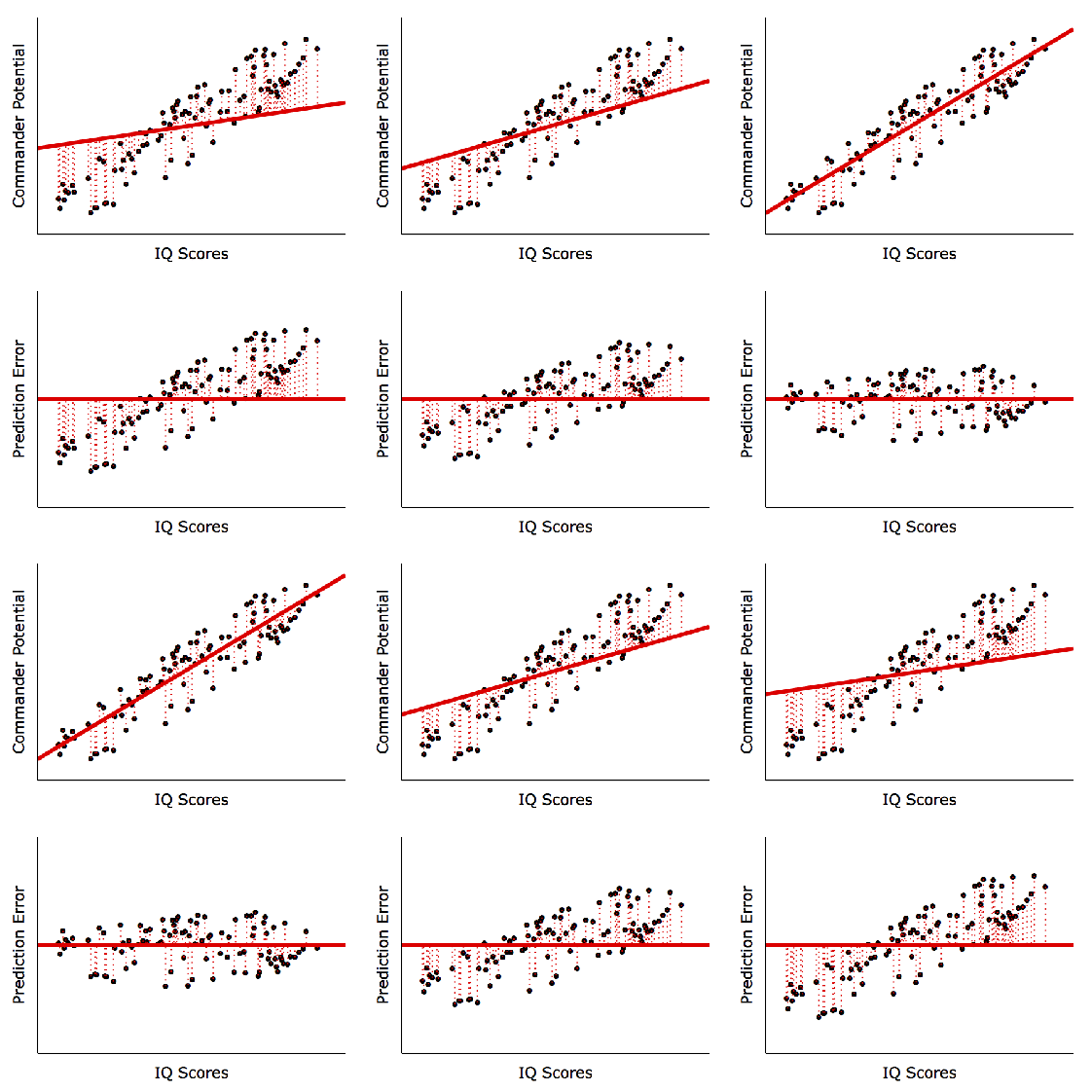
Least squares is called a loss function (for badness of fit or errors). It is not the only loss function in use. The loss function most often used by statisticians other than least squares is called maximum likelihood. Least squares is a good choice for regression lines because is has been proved that least squares provides estimates that are BLUE, that is, Best (minimum variance) Linear Unbiased Estimates of the regression line. Maximum likelihood estimates are consistent; they become less and less unbiased as the sample size increases. You will see maximum likelihood (rather than least squares) used in many multivariate applications. ML is also used in topic we will cover later, that is, logistic regression, often used in when the dependent variable is binary.
Partitioning the Sum of Squares
As we saw in Table 2, each value of weight (Y) could be thought of as a part due to the linear regression (a + bX, or Y') and a piece due to error (e, or Y-Y'). In other words, Y = Y'+e. As we saw in the table, the variance of Y equals the variance of Y' plus the variance of e. Now the variance of Y' is also called the variance due to regression and the variance of e is called the variance of error. We can work this a little more formally by considering each observed score as deviation from the mean of Y due in part to regression and in part due to error.
|
Observed |
Mean of Y |
Deviation from Mean due to Regression |
Error Part |
|
Y = |
|
(Y'- |
(Y-Y') |
Subtract the mean:

![]() (2.7)
(2.7)
(I finessed a part of the derivation that includes the cross products just before 2.7. The cross products sum to zero.)
This means that the sum of squares of Y equals the sum of squares regression plus the sum of squares of error (residual). If we divide through by N, we would have the variance of Y equal to the variance of regression plus the variance residual. For lots of work, we don't bother to use the variance because we get the same result with sums of squares and it's less work to compute them.
The big point here is that we can partition the variance or sum of squares in Y into two parts, the variance (SS) of regression and the variance (SS) of error or residual.
We can also divide through by the sum of squares Y to get a proportion:
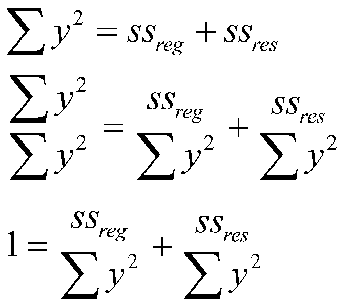 (2.8)
(2.8)
This says that the sum of squares of Y can be divided into two proportions, that due to regression, and that due to error. The two proportions must add to 1. Recall our example:
|
Wt (Y) |
|
Y- |
(Y- |
Y' |
Y'- |
(Y'- |
Resid (Y-Y') |
Resid2 |
|
105 |
150 |
-45 |
2025 |
108.19 |
-41.81 |
1748.076 |
-3.19 |
10.1761 |
|
120 |
150 |
-30 |
900 |
115.16 |
-34.84 |
1213.826 |
4.84 |
23.4256 |
|
120 |
150 |
-30 |
900 |
122.13 |
-27.87 |
776.7369 |
-2.13 |
4.5369 |
|
160 |
150 |
10 |
100 |
136.06 |
-13.94 |
194.3236 |
23.94 |
573.1236 |
|
120 |
150 |
-30 |
900 |
136.06 |
-13.94 |
194.3236 |
-16.06 |
257.9236 |
|
145 |
150 |
-5 |
25 |
156.97 |
6.97 |
48.5809 |
-11.97 |
143.2809 |
|
175 |
150 |
25 |
625 |
163.94 |
13.94 |
194.3236 |
11.06 |
122.3236 |
|
160 |
150 |
10 |
100 |
170.91 |
20.91 |
437.2281 |
-10.91 |
119.0281 |
|
185 |
150 |
35 |
1225 |
184.84 |
34.84 |
1213.826 |
0.16 |
0.0256 |
|
210 |
150 |
60 |
3600 |
205.75 |
55.75 |
3108.063 |
4.25 |
18.0625 |
|
Sum = 1500 |
1500 |
0 |
10400 |
1500.01 |
0.01 |
9129.307 |
-0.01 |
1271.907 |
|
Variance |
1155.56 |
1014.37 |
141.32 |
The total sum of squares for Y is 10400. The sum of squares for regression is 9129.31, and the sum of squares for error is 1271.91. The regression and error sums of squares add to 10401.22, which is a tad off because of rounding error. Now we can divide the regression and error sums of square by the sum of squares for Y to find proportions.

We can do the same with the variance of each:

Both formulas say that the total variance (SS) can be split into two pieces, 1 for regression, and 1 for error. The two pieces each count for a part of the variance (SS) in Y.
We can also compute simple correlation between Y and the predicted value of Y, that is, rY, Y'. For these data, that correlation is .94, which is also the correlation between X and Y (observed height and observed weight). (This is so because Y' is a linear transformation of X.) If we square .94, we get .88, which is called R-square, the squared correlation between Y and Y'. Notice that R-square is the same as the proportion of the variance due to regression: they are the same thing. We could also compute the correlation between Y and the residual, e. For our data, the resulting correlation is .35. If we square .35, we get .12, which is the squared correlation between Y and the residual, that is, rYe. This is also the proportion of variance due to error, and it agrees with the proportions we got based upon the sums of squares and variances. We could also correlate Y' with e. The result would be zero. There are two separate, uncorrelated pieces of Y, one due to regression (Y') and the other due to error (e).
Testing the Significance of the Regression and of R-square
Because R-square is the same as proportion of variance due to the regression, which is the same as the proportion of the total sum of squares due to regression, testing one of these is the same as testing for any of them. The test statistics that we will use follow the F distribution. They yield identical results because they test the same thing. To test for the significance of the regression sum of squares:
 (2.9)
(2.9)
where k is the number of independent variables or predictors, and N is the sample size. In our example, k is 1 because there is one independent variable. In our example, N is 10. The statistic computed in Equation 2.9 is a ratio of two mean squares (variance estimates), which is distributed as F with k and (N-k-1) degrees of freedom when the null hypothesis (that R-sqaure in the population is zero) is true.
In our example, the computation is:

To test for R-square, we use the formula:
 (2.10)
where N and k have the same meaning as before, and r2 is the squared correlation between Y and Y'.
In our example, the computation is:

which is the same as our earlier result within rounding error. In general, the results will be exactly the same for these two tests except for rounding error.
To anticipate a little bit, soon we will be using multiple regression, where we have more than one independent variable. In that case, instead of r (the correlation) we will have R (the multiple correlation), and instead of r2 we will have R2, so the capital R indicates multiple predictors. However, the test for R2 is the one just mentioned, that is,

So, if we had 2 independent variables and R2 was .88, F would be

