Part 3: Regression

This section mainly deals with independent variables that are continous rather than categorical. Psychologists consider many variables to be continuous that other disciplines might consider ordinal, for example, summated rating scales indicating attitudes. In my opinion, such a practice is justified not by the math, but by the consequences of doing so (i.e., things usually work pretty well if we assume interval rather than ordinal data). In this section we also cover analysis of covariance, where the model contains both continuous and categorical variables.

Correlation

This module describes the correlation coeffient, Pearson's r. It provides a couple of formulas, shows some scatterplots, describes the sampling distribution of r and the Fisher r to z transformation, describes and illustrates statistical tests involving correlelations, describes the impact of range restriction and measurement error on the correlation, and shows how to estimate statistical power for the correlation using SAS.

PowerPoint slides. Narrative description of the correlation.R code for computing corrrelations and scatterplots.

Simple Regression

This module is about linear regression with a single independent variable. In this module, we reintroduce the general linear model and the jargon that accompanies regression. After introducing the idea of the linear transformation, we show the basic idea of decomposing each score on the dependent variable into a part that is predicted by the model's independent variable and a part that is not (error or residual). Then we show how to find the regression line to satisfy the notion of least squares. Finally, we cover the significance test for R-square, that is, the test of whether the independent varialbe (predictor) accounts for any variance in the population from which our data were drawn.

PowerPoint slides. Narrative description of simple regression. R code for simple regression.

Multiple Regression

In multiple regression we have two or more indepenent variables. In this module, I mostly stick to two variables, because the equations to solve for the slopes are still more or less managable without matrix algebra. We cover how to estimation the regression equation with two independent variables with a numerical example. A second page reviews the same example using matrix algebra. The advantage of matrix algebra is that the same equation holds regardless of the number of predictors. We also show the multiple scatterplots that occur when there are two independent variables. We show how the residuals are uncorrelated with ALL of the independent variables, which anticipates partial correlation and the notion of 'holding constant' via statistics. The computation of the general formula for testing R-square is illustrated, as is the method for testing increments in R-square as various numbers of independent variables are added to the model. Standardized regression weights (sometimes called 'beta weights' are introduced.) Tests of the slopes ('b weights' or regression weights) are provided.

PowerPoint for multiple regression. R code for multiple regression. Narrative description of the material in the PowerPoint deck. Estimation of the regression equation and statistical tests using matrix algebraa.

Partial and Semipartial Correlation

Partial and semipartial correlations show the association between two focal variables when one or more peripheral variables are controlled to hold them constant through statistical means. For example, we might want to know the correlation between job satisfaction and autonomy at work holding constant a measure of negative affect or social desirability. The partial and semipartial correlations can be computed using residuals from regression analysis (and also by simpler means). The regression slope is closely related to the semipartial correlation.

PowerPoint slides. Narrative description of materials in the PowerPoint deck. R code for computing partial and semipartial correlations.

Prediction

One of the main uses of regression is making point predictions. For example, given information about high school GPA, standardized test scores, and personality tests, a college can use a regression equation to make an exact prediction of a student's grade point average the end of the first year if that student is admitted. How well regression works at doing so is an important topic for this module. We cover confidence interals for the regression line and for the individual. The R-square statistic is biased, so we cover the expected shrinkage in R-square when the regression equation is applied in a new sample, both based on shrinkage formulas and taken from empirical estimates based on cross-validation. Then we describe predictor selection algorithms such as stepwise regression that are supposed to help you choose a subset of predictors to use in a given application. We contrast the predictor selection alogorithms with theory-based tests embodied in hierarchical regression tests.

PowerPoint slides. Narrative description for prediction materials covered in the PowerPoint slides.[not yet:] R code for a mixed design, two factors with one repeated (dial shape and calibration effects on errors in the choice of stove-top controls).

Indices of Variable 'Importance'

Everybody seems to want to know which variables are most important in a regression equation. When the independent variables are uncorrelated, the correlations between each predictor and the criterion provide a good index of the magnitude of the association ('importance') because the correlations will be the slopes of the standardized variables. Some people would prefer to square the correlation, because then we are talking shared variance. Unfortunately, in nonexperimental contexts, the predictors are intercorrelated, and the simple approach doesn't work well. In such cases, there multiple definitions of importance, and they may disagree substantially. I'll show you several, including dominance analysis. In my opinion, none of them does an entirely satisfactory job of defining and measuring importance.

PowerPoint slide show. Narrative description. R code for some of the computations including dominance analysis (average increment).

Regression Diagnostics (model fit, estimation problems)

We use a model to represent the data. If the model is a good representation, then our inferences should be sound. There are assumptions that are important for interpreting the results and making inferences. We describe using graphs to spot problems of outliers, heteroscedasticity and linearity. We describe computer-generated indices of model fit including studentized residuals, and dfbetas. We proceed to define collinearity (the problem of large correlations among our predictors) and indices designed to diagnose it, including tolerance, the variance inflation factor, and the condition index. I briefly describe some remedies for problems encountered by diagnostics.

Powerpoint slides. A narrative description of the material included in the slides. R code for univariate diagnostics and collinearity.

Nonlinear Relations (curves and interactions)

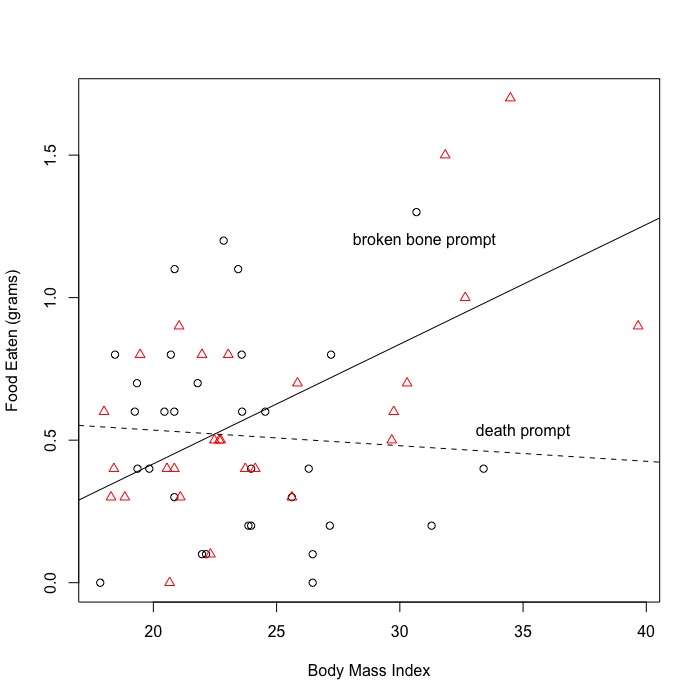
The regression model assumes that the relations between the criterion and the predictors are well represented by straight lines. Sometimes this is not the case, for example, gas mileage and engine power in automobile engines are best represented by a curved line rather than a straight one. Sometimes there are interactions among our independent variables such that the slope of one variable depends upon the value of another. For example, the relations between autonomy and job satisfaction is thought to depend upon a personality characteristic (growth need strength). Such departures from linearity are the topic of this module. First we cover polynomial regression, where we fit bends using predictors taken to powers (e.g., x and x-squared). Then we show how to test for interactions, and we end by distinguishing moderator and mediator in regression.

PowerPoint slides. R code for polynomial regression and testing interactions.

Analysis of Covariance (ANCOVA)

The analysis of covariance model contains both categorical and continuous variables. An example might test whether men or women (categorical variable) show better performance on a test at the end of a calculus class (dependent variable), where at the beginning of the class, all were given a test of quantitative reasoning (covariate). Some experimental psychologists reserve the term 'analysis of covariance' for designs in which the independent variable is randomly assigned and the covariates are used to improve power by removing nuisance variance. I don't make that distinction - here we are talking about the analsysis, not the design. However, it certainly the case that covariates can either increase or decrease the power of the test of the categorical variable, so you should be thoughtful about what goes into the model.

PowerPoint slides. R code for computing ANCOVA.